Materials Science Data Visualization Guide

Every materials scientist knows the drill: run 50 XRD scans, export data to Excel, spend hours manually stacking patterns and aligning peaks. Then a colleague asks you to replot with different color schemes for the manuscript revision. There is a better way.
This guide covers the essential visualizations for materials characterization with live Python code editors you can modify and run instantly.
What You Will Learn
0.Live Code Lab: Stress-Strain Curve
1.X-Ray Diffraction (XRD) Patterns
2.Stress-Strain & Mechanical Testing
3.Thermal Analysis (TGA/DSC)
4.Particle Size Distributions
5.Spectroscopy (FTIR / UV-Vis)
6.Live Code Lab: XRD Stacked Plot
What You'll Learn
0.Live Code Lab: Stress-Strain Curve
1.X-Ray Diffraction (XRD) Patterns
2.Stress-Strain & Mechanical Testing
3.Thermal Analysis (TGA/DSC)
4.Particle Size Distributions
5.Spectroscopy (FTIR / UV-Vis)
6.Live Code Lab: XRD Stacked Plot
0. Live Code Lab: Stress-Strain Curve
This code compares stress-strain curves for two materials, annotating the yield point, UTS, and 0.2% offset line. The code handles elastic, plastic, and necking regions.
Try changing the Young's modulus or adding a third material to the comparison.
1. X-Ray Diffraction (XRD) Patterns
The challenge with XRD data is comparing multiple samples without the plot becoming a messy spaghetti chart. The solution is a stacked (waterfall) plot with vertical offsets.
Stacked Layout
Add a vertical offset to each scan so patterns do not overlap. Use a subtle fill to separate them visually.
Peak Labels
Annotate key diffraction angles (2-theta) directly on the plot. Mark new phase peaks with a symbol.
No Y-Axis Ticks
XRD intensity is arbitrary - remove Y-axis tick labels. Label as "Intensity (a.u.)" and hide the scale.
Pro Tip
For peak-shift analysis (e.g., doping studies), add a vertical dashed line at the reference peak position so readers can immediately see the angular shift.
2. Stress-Strain & Mechanical Testing
Stress-strain plots need careful attention to units and key markers. Reviewers expect clear identification of elastic modulus, yield point, and ultimate tensile strength.
Try it
Try it now: turn this method into your next figure
Apply the same approach to your own dataset and generate clean, publication-ready code and plots in minutes.
Open in Plotivy Analyze →Newsletter
Get a weekly Python plotting tip
One concise tip each week for cleaner, faster scientific figures. Built for researchers who publish.
0.2% Offset Method
For materials without a clear yield point (like aluminum alloys), draw a line parallel to the elastic region offset by 0.2% strain. The intersection defines the yield stress.
Unit Consistency
Ensure units are consistent throughout - MPa vs GPa matters. Mark fracture, yield, and UTS with distinct annotation styles so reviewers can identify them instantly.
3. Thermal Analysis (TGA/DSC)
TGA and DSC often need to be plotted together to correlate weight loss with thermal events. The key is aligning temperature axes while keeping each technique's data readable.
Stacked Multi-Panel Figure
- Align the X-axis (Temperature) for both plots using
sharex=True - Place TGA on top (weight % vs T) and DSC on the bottom (heat flow vs T)
- Mark onset temperatures with vertical dashed lines that span both panels
- Annotate weight loss percentages directly on the TGA curve
Try it: Upload TGA/DSC data and ask "Create a two-panel thermal analysis plot with aligned temperature axes".
4. Particle Size Distributions
Whether from DLS or image analysis, particle size data is best shown as a histogram + cumulative distribution on dual axes.
Histogram + CDF
Plot the frequency histogram on the left Y-axis and the cumulative percentage curve (S-curve) on the right. Mark D10, D50, D90 values with horizontal lines.
Log-Normal Fit
Most particle size distributions are log-normal. Overlay the fitted distribution on a log-scale X-axis to validate your data quality.
5. Spectroscopy (FTIR / UV-Vis)
FTIR Convention
Plot wavenumber on the X-axis in decreasing order (4000 to 400 cm-1). Most journals expect transmittance (%) on the Y-axis, though absorbance is also acceptable.
UV-Vis for Materials
Plot wavelength increasing left to right. For bandgap determination, create a Tauc plot inset: (alpha*hv)^n vs hv, where n=2 for direct and n=0.5 for indirect bandgaps.
Stop wasting hours on XRD and TGA plots
Describe what you need and get publication-ready figures with one prompt. Plotivy handles stacked XRD, dual-axis thermal analysis, and stress-strain annotations automatically.
6. Live Code Lab: XRD Stacked Plot
This code creates a stacked XRD waterfall plot comparing three samples with different phases. New phase peaks are marked with symbols and key diffraction angles are labeled.
Try adding additional peaks, changing peak widths, or modifying the vertical offset to create your own comparison.
Chart gallery
Materials science chart templates
Start from these gallery examples and customize for your XRD, thermal, or mechanical testing data.

Line Graph
Displays data points connected by straight line segments to show trends over time.
Sample code / prompt
import matplotlib.pyplot as plt
import numpy as np

# Generate temperature data for 3 major US cities over 12 months
months = ['Jan', 'Feb', 'Mar', 'Apr', 'May', 'Jun', 'Jul', 'Aug', 'Sep', 'Oct', 'Nov', 'Dec']
nyc = [30, 32, 40, 52, 65, 75, 82, 81, 74, 63, 50, 38]
miami = [65, 66, 70, 76, 82, 87, 90, 90, 87, 80, 72, 66]
chicago = [25, 27, 35, 48, 62, 72, 80, 79, 71, 60, 45, 32]

# Create figure with enhanced styling
Heatmap
Represents data values as colors in a two-dimensional matrix format.
Sample code / prompt
import matplotlib.pyplot as plt
import seaborn as sns
import pandas as pd
import numpy as np

# Create correlation matrix for financial metrics
metrics = ['Revenue', 'Profit', 'Expenses', 'ROI', 'Customers', 'AOV', 'Marketing', 'Employees']
correlation_data = np.array([
    [1.00, 0.85, -0.45, 0.72, 0.88, 0.65, 0.72, 0.55],
    [0.85, 1.00, -0.78, 0.92, 0.75, 0.58, 0.63, 0.48],
Scatterplot
Displays values for two variables as points on a Cartesian coordinate system.
Sample code / prompt
import matplotlib.pyplot as plt
import numpy as np
from scipy import stats
import pandas as pd

# Generate sample data
np.random.seed(42)
n_samples = 200
height = np.random.normal(170, 8, n_samples)
weight = height * 0.6 + np.random.normal(0, 8, n_samples) - 50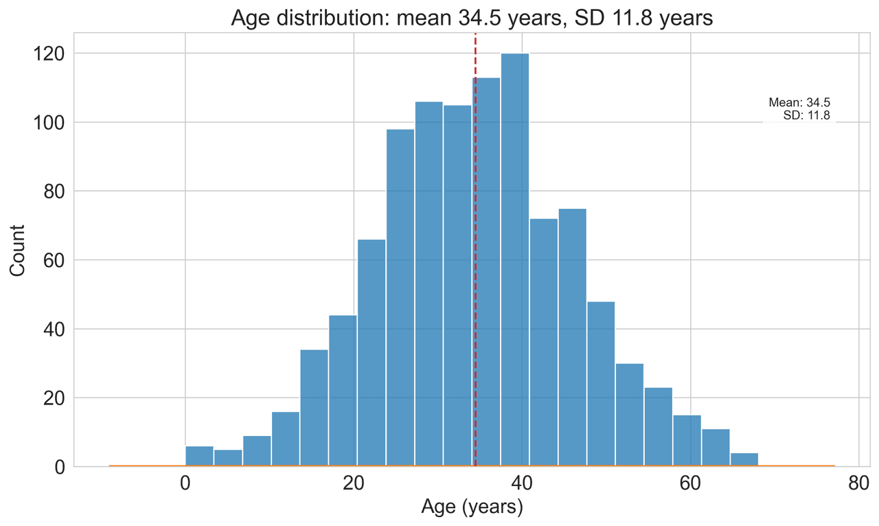
Histogram
Displays the distribution of numerical data by grouping values into bins.
Sample code / prompt
import matplotlib.pyplot as plt
import numpy as np
from scipy.stats import gaussian_kde, skewnorm

# Generate age data with slight right skew
np.random.seed(42)
ages = skewnorm.rvs(a=2, loc=42, scale=15, size=500)
ages = np.clip(ages, 18, 80)  # Clip to realistic range

fig, ax = plt.subplots(figsize=(12, 7))Visualize Your Materials Data Now
Upload XRD, TGA, stress-strain, or spectroscopy data. Describe the plot you want and get publication-ready Python code instantly.
Technique guides scientists read next
scipy.signal.find_peaks guide
Tune prominence and width parameters for robust peak extraction.
Savitzky-Golay smoothing
Reduce noise while preserving peak shape and position.
PCA visualization workflow
Move from high-dimensional measurements to interpretable components.
ANOVA with post-hoc brackets
Add statistically correct pairwise significance annotations.
Found this helpful? Share it with your network.
Experimental Physicist & Photonics Researcher
Hands-on experience in silicon photonics, semiconductor fabrication (DRIE/ICP-RIE), optical simulation, and data-driven analysis. Built Plotivy to help researchers focus on discoveries instead of data struggles.
More about the authorVisualize your own data
Apply the techniques from this article to your own datasets. Upload CSV, Excel, or paste data directly.