How to Remove Legend Title in ggplot2 (The Easy Way)

The ggplot2 legend title is the most Googled thing to remove in R. Here is every method, plus the Python/Matplotlib equivalents so you can do it in either language.
Quick Reference
0.Live Code: Legend Customization
1.Remove Legend Title (theme())
2.Remove Entire Legend
3.Per-Scale Control (guides())
4.Rename Instead of Remove
0. Live Code: Legend Customization
Three legend styles side by side: with title, without title, and direct labels. The Python/Matplotlib equivalents of ggplot2 legend controls.
1. Remove Legend Title with theme()
R / ggplot2
ggplot(df, aes(x, y, color = group)) +
  geom_point() +
  theme(legend.title = element_blank())
element_blank() removes the title while keeping the legend entries. This is the most common approach.
Try it
Try it now: turn this method into your next figure
Apply the same approach to your own dataset and generate clean, publication-ready code and plots in minutes.
Open in Plotivy Analyze →Newsletter
Get a weekly Python plotting tip
One concise tip each week for cleaner, faster scientific figures. Built for researchers who publish.
2. Remove the Entire Legend
R / ggplot2
ggplot(df, aes(x, y, color = group)) +
  geom_point() +
  theme(legend.position = "none")
When to Remove
Remove legends when using direct labels on the data, in faceted plots where the title is self-explanatory, or when the groups are obvious from context.
3. Per-Scale Control with guides()
R / ggplot2
ggplot(df, aes(x, y, color = group, size = value)) +
  geom_point() +
  guides(color = guide_legend(title = NULL),   # remove color title
         size = guide_legend(title = "Value"))  # keep size title
Use guides() when you have multiple scales and want to remove only specific legend titles.
4. Rename Instead of Remove
R / ggplot2
ggplot(df, aes(x, y, color = group)) +
  geom_point() +
  labs(color = "Treatment Group")   # rename instead
Chart gallery
Related chart types
Explore chart types where legend management matters most.

Scatterplot
Displays values for two variables as points on a Cartesian coordinate system.
Sample code / prompt
import matplotlib.pyplot as plt
import numpy as np
from scipy import stats
import pandas as pd

# Generate sample data
np.random.seed(42)
n_samples = 200
height = np.random.normal(170, 8, n_samples)
weight = height * 0.6 + np.random.normal(0, 8, n_samples) - 50
Line Graph
Displays data points connected by straight line segments to show trends over time.
Sample code / prompt
import matplotlib.pyplot as plt
import numpy as np

# Generate temperature data for 3 major US cities over 12 months
months = ['Jan', 'Feb', 'Mar', 'Apr', 'May', 'Jun', 'Jul', 'Aug', 'Sep', 'Oct', 'Nov', 'Dec']
nyc = [30, 32, 40, 52, 65, 75, 82, 81, 74, 63, 50, 38]
miami = [65, 66, 70, 76, 82, 87, 90, 90, 87, 80, 72, 66]
chicago = [25, 27, 35, 48, 62, 72, 80, 79, 71, 60, 45, 32]

# Create figure with enhanced styling
Bar Chart
Compares categorical data using rectangular bars with heights proportional to values.
Sample code / prompt
import numpy as np
import pandas as pd
import matplotlib.pyplot as plt
import seaborn as sns
from scipy import stats

# Generate performance scores for 5 treatment groups
np.random.seed(42)
groups = ['Control', 'Treatment A', 'Treatment B', 'Treatment C', 'Treatment D']
n_samples = 30.png&w=1280&q=70)
Box and Whisker Plot
Displays data distribution using quartiles, median, and outliers in a standardized format.
Sample code / prompt
import numpy as np
import pandas as pd
import matplotlib.pyplot as plt
import seaborn as sns
from scipy import stats

# Generate gene expression data for 4 genotypes
np.random.seed(42)
genotypes = ['WT', 'KO1', 'KO2', 'Mutant']
n_per_group = 20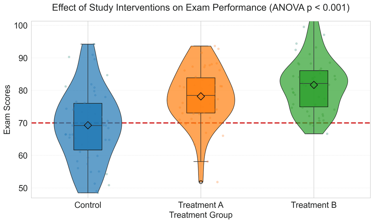
Violin Plot
Combines box plots with kernel density to show distribution shape across groups.
Sample code / prompt
import matplotlib.pyplot as plt
import seaborn as sns
import pandas as pd
import numpy as np
from scipy.stats import f_oneway

# Generate exam score data for 3 groups
np.random.seed(42)
control = np.random.normal(72, 12, 50)
treatment_a = np.random.normal(78, 10, 50)Automate R Legend Formatting
Upload your data, toggle to R language mode, and type "remove legend title". Plotivy generates the correct theme or guides code and renders the figure instantly.
Technique guides scientists read next
scipy.signal.find_peaks guide
Tune prominence and width parameters for robust peak extraction.
Savitzky-Golay smoothing
Reduce noise while preserving peak shape and position.
PCA visualization workflow
Move from high-dimensional measurements to interpretable components.
ANOVA with post-hoc brackets
Add statistically correct pairwise significance annotations.
Found this helpful? Share it with your network.
Experimental Physicist & Photonics Researcher
Hands-on experience in silicon photonics, semiconductor fabrication (DRIE/ICP-RIE), optical simulation, and data-driven analysis. Built Plotivy to help researchers focus on discoveries instead of data struggles.
More about the authorVisualize your own data
Apply the techniques from this article to your own datasets. Upload CSV, Excel, or paste data directly.