How to Create Publication-Ready Figures in Under 10 Minutes

How much of your PhD have you spent adjusting axis labels? Creating figures for a manuscript often means hours of tweaking font sizes, fighting with color palettes, and redoing everything when your advisor asks for "minor changes."
This guide walks you through the complete workflow with live Python code editors so you can see publication styling in action.
What You Will Learn
0.Live Code Lab: Before & After
1.Step 1 - Upload Your Data
2.Step 2 - Generate the Plot
3.Step 3 - Apply Publication Styling
4.Step 4 - Export High-Res Assets
5.Why This Beats the Old Way
6.Start with a Template
0. Live Code Lab: Publication-Ready Scatter Plot
This code creates a complete publication-ready calibration curve - Beer-Lambert data with error bars, linear regression, R-squared, and clean journal styling (Arial font, removed top/right spines).
Modify the font size, colors, or marker styles to match your target journal's requirements.
The 10-Minute Workflow
The Promise
Follow this workflow to create a figure that meets Nature/Science guidelines in less time than it takes to drink your coffee.
1. Upload Your Data (Minute 0-2)
Upload a clean CSV or Excel file. The AI can handle messy headers, but cleaner data means better results.
2. Generate the Plot (Minute 2-5)
Describe your plot in plain English. Be specific about variables, plot type, and any statistics.
The more specific your prompt, the fewer iterations you need. Include column names, units, and the type of statistics you want.
Try it
Try it now: review your figure before submission
Upload your current plot and get an AI critique with concrete fixes for clarity, typography, color, and journal readiness.
Open AI Figure Reviewer →Newsletter
Get a weekly Python plotting tip
One concise tip each week for cleaner, faster scientific figures. Built for researchers who publish.
3. Apply Publication Styling (Minute 5-8)
Apply specific journal requirements in a single refinement prompt.
See the difference styling makes:


Slide to compare default output vs. publication-ready styling.
4. Export High-Res Assets (Minute 8-10)
PNG (300 DPI)
For manuscript drafts and presentations. Set dpi=300 for print quality.
SVG / PDF
Vector formats for final submission. Text remains editable and scales to any size without pixelation.
Python Code
Download the generated code for reproducibility. Include it in your supplementary materials.
5. Why This Beats the Old Way
Reproducibility
Unlike point-and-click software where steps are lost, Plotivy generates Python code. You have a permanent audit trail of exactly how the figure was created.
Vector Quality
We export native SVG/PDF via Matplotlib, ensuring your Nature paper looks crisp at any zoom level - unlike screenshots from Excel or GraphPad.
Try the 10-Minute Challenge
Upload a dataset and see if you can beat the clock. Most users get their first publication-ready figure in under 2 minutes.
Bonus: Multi-Panel Publication Figure
Most manuscripts need multi-panel figures. This code creates a 2x2 layout with consistent styling across all panels - line plot, bar chart, scatter, and box plot.
Try changing the layout to 1x4 or 3x2, or switch the plot types to match your data.
6. Start with a Template
Do not even want to write a prompt? Click one of these to start with a pre-made publication-quality template.
Chart gallery
Publication-ready chart templates
Start from these gallery templates - each one follows journal styling guidelines out of the box.

Scatterplot
Displays values for two variables as points on a Cartesian coordinate system.
Sample code / prompt
import matplotlib.pyplot as plt
import numpy as np
from scipy import stats
import pandas as pd

# Generate sample data
np.random.seed(42)
n_samples = 200
height = np.random.normal(170, 8, n_samples)
weight = height * 0.6 + np.random.normal(0, 8, n_samples) - 50
Line Graph
Displays data points connected by straight line segments to show trends over time.
Sample code / prompt
import matplotlib.pyplot as plt
import numpy as np

# Generate temperature data for 3 major US cities over 12 months
months = ['Jan', 'Feb', 'Mar', 'Apr', 'May', 'Jun', 'Jul', 'Aug', 'Sep', 'Oct', 'Nov', 'Dec']
nyc = [30, 32, 40, 52, 65, 75, 82, 81, 74, 63, 50, 38]
miami = [65, 66, 70, 76, 82, 87, 90, 90, 87, 80, 72, 66]
chicago = [25, 27, 35, 48, 62, 72, 80, 79, 71, 60, 45, 32]

# Create figure with enhanced styling
Bar Chart
Compares categorical data using rectangular bars with heights proportional to values.
Sample code / prompt
import numpy as np
import pandas as pd
import matplotlib.pyplot as plt
import seaborn as sns
from scipy import stats

# Generate performance scores for 5 treatment groups
np.random.seed(42)
groups = ['Control', 'Treatment A', 'Treatment B', 'Treatment C', 'Treatment D']
n_samples = 30
Error Bars
Graphical representations of the variability of data indicating error or uncertainty in measurements.
Sample code / prompt
import numpy as np
import matplotlib.pyplot as plt
from scipy import stats

# Generate bacterial growth data with replicates
np.random.seed(42)
time_points = np.array([0, 4, 8, 12, 18, 24])
mean_values = np.array([10, 25, 80, 250, 600, 800])

# Generate 5 replicates per time point with noise.png&w=1280&q=70)
Box and Whisker Plot
Displays data distribution using quartiles, median, and outliers in a standardized format.
Sample code / prompt
import numpy as np
import pandas as pd
import matplotlib.pyplot as plt
import seaborn as sns
from scipy import stats

# Generate gene expression data for 4 genotypes
np.random.seed(42)
genotypes = ['WT', 'KO1', 'KO2', 'Mutant']
n_per_group = 20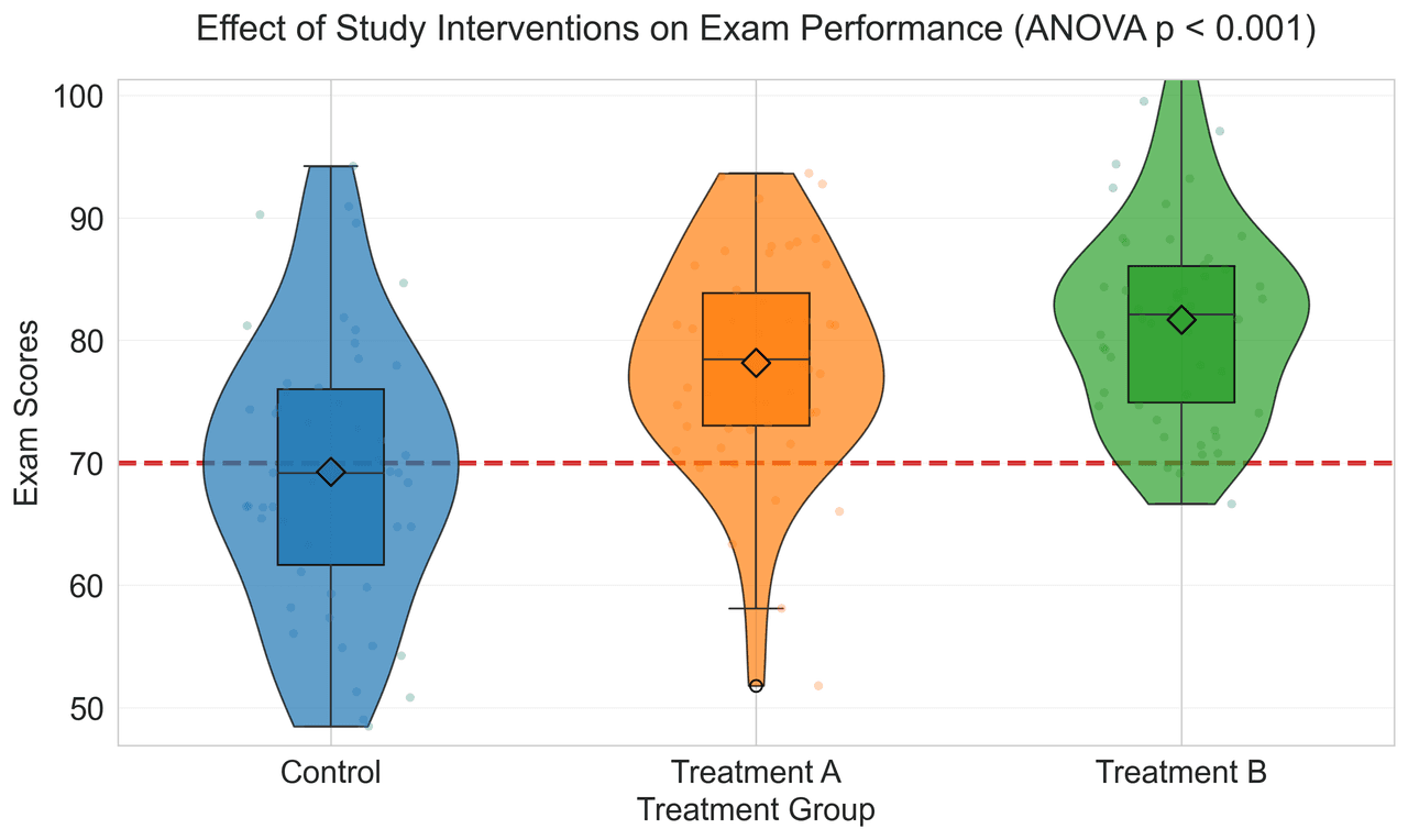
Violin Plot
Combines box plots with kernel density to show distribution shape across groups.
Sample code / prompt
import matplotlib.pyplot as plt
import seaborn as sns
import pandas as pd
import numpy as np
from scipy.stats import f_oneway

# Generate exam score data for 3 groups
np.random.seed(42)
control = np.random.normal(72, 12, 50)
treatment_a = np.random.normal(78, 10, 50)Get Your First Figure in 2 Minutes
Upload your data, describe what you want, and let Plotivy generate publication-ready Python code instantly.
Technique guides scientists read next
scipy.signal.find_peaks guide
Tune prominence and width parameters for robust peak extraction.
Savitzky-Golay smoothing
Reduce noise while preserving peak shape and position.
PCA visualization workflow
Move from high-dimensional measurements to interpretable components.
ANOVA with post-hoc brackets
Add statistically correct pairwise significance annotations.
Found this helpful? Share it with your network.
Experimental Physicist & Photonics Researcher
Hands-on experience in silicon photonics, semiconductor fabrication (DRIE/ICP-RIE), optical simulation, and data-driven analysis. Built Plotivy to help researchers focus on discoveries instead of data struggles.
More about the authorVisualize your own data
Apply the techniques from this article to your own datasets. Upload CSV, Excel, or paste data directly.