R vs Python for Data Science: The Complete 2026 Comparison

R vs Python is the oldest debate in data science. The honest answer: both are excellent, and the best choice depends on your field, your lab, and your career goals. Here is the unbiased comparison.
In This Comparison
0.Live Code: Python Scientific Figure
1.Language Philosophy
2.Feature Comparison Table
3.When R Wins
4.When Python Wins
5.Code Comparison
6.Which Should You Learn?
0. Live Code: PCA Biplot in Python
PCA biplot with 95% confidence ellipses - a multivariate analysis figure that R handles with ggbiplot and Python handles with matplotlib. Edit and re-run below.
1. Language Philosophy
R: Statistics-First
R was built by statisticians for statisticians. Everything is a vector. Data frames are first-class citizens. Statistical tests are one-liners.
Created: 1993 by Ross Ihaka and Robert Gentleman
Python: General-Purpose
Python was built as a readable general-purpose language. Data science capabilities come from libraries (numpy, pandas, scipy, matplotlib).
Created: 1991 by Guido van Rossum
2. Feature Comparison Table
| Category | R | Python |
|---|---|---|
| Statistical testing | Built-in (t.test, aov, lm) | scipy.stats, statsmodels |
| Visualization | ggplot2 (Grammar of Graphics) | matplotlib, seaborn, plotly |
| Machine learning | caret, tidymodels | scikit-learn, PyTorch, TF |
| Data manipulation | dplyr, tidyr (tidyverse) | pandas, polars |
| Genomics/Bioinformatics | Bioconductor (excellent) | Biopython (basic) |
| Reproducible reports | RMarkdown, Quarto | Jupyter, Quarto |
| Job market (industry) | Smaller | Much larger |
| Job market (academia) | Strong (stats, bio) | Strong (CS, physics, eng) |
| Learning curve | Medium (unique syntax) | Low-medium (readable syntax) |
3. When R Wins
Genomics & Bioinformatics
Bioconductor has 2,000+ packages for RNA-seq, ChIP-seq, variant calling.
Statistical Modeling
Mixed-effects models (lme4), Bayesian inference (brms, Stan) are more mature.
Publication Plots
ggplot2 produces beautiful multi-faceted plots with minimal code.
Epidemiology
survival, epiR, EpiEstim packages are the gold standard.
Try it
Try it now: turn this method into your next figure
Apply the same approach to your own dataset and generate clean, publication-ready code and plots in minutes.
Open in Plotivy Analyze →Newsletter
Get a weekly Python plotting tip
One concise tip each week for cleaner, faster scientific figures. Built for researchers who publish.
4. When Python Wins
Machine Learning / Deep Learning
scikit-learn, PyTorch, TensorFlow. The entire ML ecosystem is Python-first.
Automation & Pipelines
General-purpose language = web scraping, API calls, file processing in one script.
Industry Jobs
Python is the #1 language in data science job postings by a wide margin.
Large-Scale Data
Better memory management. Polars and Dask handle billion-row datasets.
5. Code Comparison
R + ggplot2
library(ggplot2)

ggplot(df, aes(x=dose, y=response,
               color=treatment)) +
  geom_point(size=3) +
  geom_smooth(method="lm") +
  theme_minimal() +
  labs(title="Dose-Response",
       x="Dose (mg/kg)",
       y="Response (%)")
Python + matplotlib
import matplotlib.pyplot as plt
import numpy as np

for t in treatments:
    mask = df["treatment"] == t
    plt.scatter(df[mask]["dose"],
                df[mask]["response"],
                label=t, s=30)
plt.xlabel("Dose (mg/kg)")
plt.ylabel("Response (%)")
plt.legend()
plt.title("Dose-Response")
6. Which Should You Learn?
You are in biology, epidemiology, or social science
Start with RYou want industry data science jobs
Start with PythonYour PI or lab uses one language
Use what the lab usesYou want publication figures fastest
Plotivy (AI + Python)You plan to do deep learning
PythonYou want both - which first?
Python (broader utility)7. The Best of Both Worlds: Plotivy Supports R and Python
You no longer have to choose between languages just to make a quick figure. Plotivy provides sandboxed execution engines for both Python (Matplotlib and Plotly) and R (ggplot2).
Switching Languages is Easy
Simply toggle the language switcher above the prompt input inside the analyzer. Upload a CSV file and ask the AI in plain English: "create a scatter plot using ggplot2 with theme_classic()" or "fit a linear regression with matplotlib".
Try the R / ggplot2 AnalyzerChart gallery
Skip the Syntax - Use AI
Generate publication-ready Python figures without memorizing matplotlib APIs.

Scatterplot
Displays values for two variables as points on a Cartesian coordinate system.
Sample code / prompt
import matplotlib.pyplot as plt
import numpy as np
from scipy import stats
import pandas as pd

# Generate sample data
np.random.seed(42)
n_samples = 200
height = np.random.normal(170, 8, n_samples)
weight = height * 0.6 + np.random.normal(0, 8, n_samples) - 50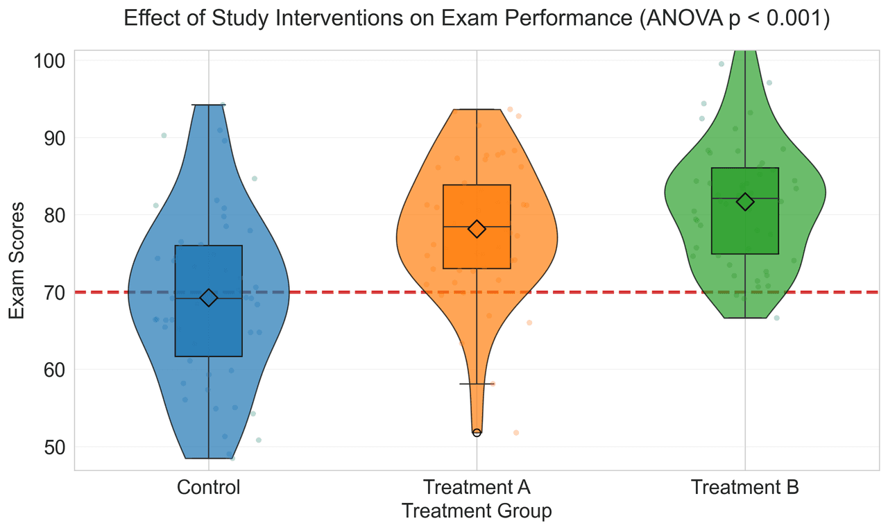
Violin Plot
Combines box plots with kernel density to show distribution shape across groups.
Sample code / prompt
import matplotlib.pyplot as plt
import seaborn as sns
import pandas as pd
import numpy as np
from scipy.stats import f_oneway

# Generate exam score data for 3 groups
np.random.seed(42)
control = np.random.normal(72, 12, 50)
treatment_a = np.random.normal(78, 10, 50)
Heatmap
Represents data values as colors in a two-dimensional matrix format.
Sample code / prompt
import matplotlib.pyplot as plt
import seaborn as sns
import pandas as pd
import numpy as np

# Create correlation matrix for financial metrics
metrics = ['Revenue', 'Profit', 'Expenses', 'ROI', 'Customers', 'AOV', 'Marketing', 'Employees']
correlation_data = np.array([
    [1.00, 0.85, -0.45, 0.72, 0.88, 0.65, 0.72, 0.55],
    [0.85, 1.00, -0.78, 0.92, 0.75, 0.58, 0.63, 0.48],
Bar Chart
Compares categorical data using rectangular bars with heights proportional to values.
Sample code / prompt
import numpy as np
import pandas as pd
import matplotlib.pyplot as plt
import seaborn as sns
from scipy import stats

# Generate performance scores for 5 treatment groups
np.random.seed(42)
groups = ['Control', 'Treatment A', 'Treatment B', 'Treatment C', 'Treatment D']
n_samples = 30
Error Bars
Graphical representations of the variability of data indicating error or uncertainty in measurements.
Sample code / prompt
import numpy as np
import matplotlib.pyplot as plt
from scipy import stats

# Generate bacterial growth data with replicates
np.random.seed(42)
time_points = np.array([0, 4, 8, 12, 18, 24])
mean_values = np.array([10, 25, 80, 250, 600, 800])

# Generate 5 replicates per time point with noise
Line Graph
Displays data points connected by straight line segments to show trends over time.
Sample code / prompt
import matplotlib.pyplot as plt
import numpy as np

# Generate temperature data for 3 major US cities over 12 months
months = ['Jan', 'Feb', 'Mar', 'Apr', 'May', 'Jun', 'Jul', 'Aug', 'Sep', 'Oct', 'Nov', 'Dec']
nyc = [30, 32, 40, 52, 65, 75, 82, 81, 74, 63, 50, 38]
miami = [65, 66, 70, 76, 82, 87, 90, 90, 87, 80, 72, 66]
chicago = [25, 27, 35, 48, 62, 72, 80, 79, 71, 60, 45, 32]

# Create figure with enhanced stylingFrequently Asked Questions
Should I learn R or Python in 2026?
Is ggplot2 better than matplotlib for scientific figures?
Can I use both R and Python in the same project?
Is R dying or being replaced by Python?
What is the fastest way to create scientific plots without learning R or Python?
Python Figures Without the Learning Curve
Describe your figure in English, get editable Python code, export at 600 DPI.
Technique guides scientists read next
scipy.signal.find_peaks guide
Tune prominence and width parameters for robust peak extraction.
Savitzky-Golay smoothing
Reduce noise while preserving peak shape and position.
PCA visualization workflow
Move from high-dimensional measurements to interpretable components.
ANOVA with post-hoc brackets
Add statistically correct pairwise significance annotations.
Found this helpful? Share it with your network.
Experimental Physicist & Photonics Researcher
Hands-on experience in silicon photonics, semiconductor fabrication (DRIE/ICP-RIE), optical simulation, and data-driven analysis. Built Plotivy to help researchers focus on discoveries instead of data struggles.
More about the authorVisualize your own data
Apply the techniques from this article to your own datasets. Upload CSV, Excel, or paste data directly.