Menu

Dimensionality Reduction

Interactive PCA Biplots Made Simple

Principal Component Analysis compresses high-dimensional data into interpretable 2D projections. Plotivy generates PCA biplots with confidence ellipses, loading vectors, and scree plots from a single dataset upload.

Understanding PCA in 60 Seconds

PCA finds a new coordinate system where the first axis (PC1) captures the most variance, the second axis (PC2) captures the next most, and so on. It is used across every scientific discipline - from genomics to materials science - to find patterns in complex datasets.

Scores

Sample positions in PC space - points in the biplot

Loadings

Feature contributions - arrows showing how variables drive separation

Eigenvalues

Variance captured by each PC - shown in scree plots

Ellipses

95% confidence regions - indicate cluster overlap or separation

Live Code Lab: PCA Biplot

This code performs PCA from scratch (no sklearn) on a 4-feature dataset, then creates a publication-quality biplot with confidence ellipses and loading vectors.

Key customization tips

  • Add groups: add more arrays like group_d and extend the labels list
  • Change features: modify feature names and adjust the data generation parameters
  • Remove loadings: comment out the loading vector section for a scores-only plot
  • 3D PCA: use from mpl_toolkits.mplot3d import Axes3D and project onto 3 PCs

PCA Across Scientific Fields

Genomics / Transcriptomics

Population stratification from SNP data, sample QC in RNA-seq

Chemistry / Spectroscopy

Identify compound types from FTIR, NMR, or Raman spectra

Materials Science

Correlate mechanical, thermal, and compositional properties

Ecology / Environmental

Community composition analysis from species abundance data

Food Science / Agriculture

Quality classification from sensory or chemical profiles

Clinical / Biomarkers

Patient stratification from multi-panel blood analyses

Bonus: Scree Plot

Always include a scree plot alongside your PCA biplot. It shows how many components to retain - look for the "elbow" where eigenvalues flatten.

Why Use Plotivy for PCA

Automatic scaling & centering

Plotivy detects whether your features need z-score normalization or unit-variance scaling and applies it before decomposition.

Confidence ellipses

95% confidence regions are drawn automatically for each group, making cluster separation visually obvious.

Explained variance labels

Axis labels automatically show the percentage of variance captured by each PC - no manual calculation needed.

Publication-ready export

Download biplots and scree plots at 300+ DPI with Arial fonts and proper sizing for any journal.

Chart gallery

Related Multivariate Charts

Other ways to explore high-dimensional data

Browse all chart types →
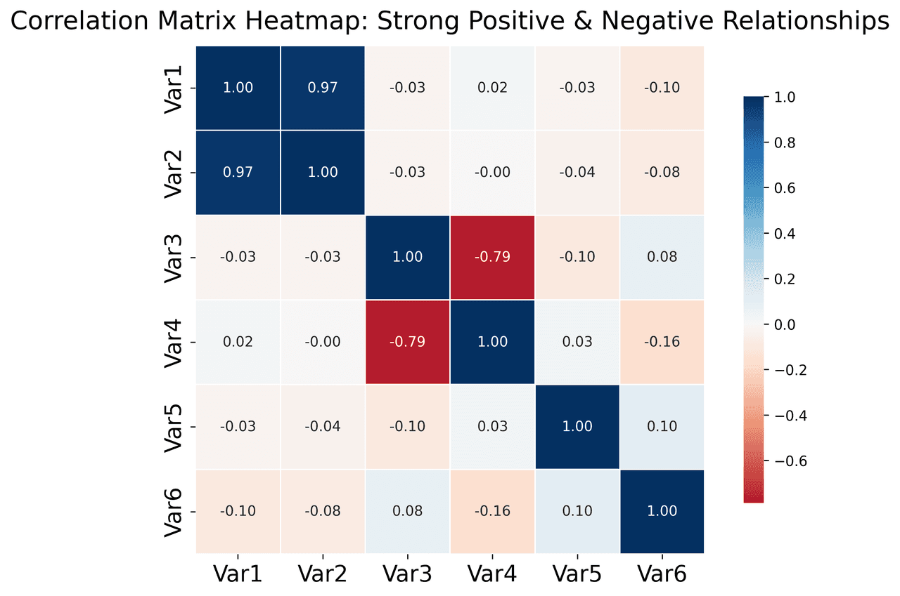
Correlation heatmap with diverging color scale and coefficient annotations
Statistical•seaborn, matplotlib
From the chart gallery•Correlation analysis between variables

Heatmap

Represents data values as colors in a two-dimensional matrix format.

Sample code / prompt

import matplotlib.pyplot as plt
import seaborn as sns
import pandas as pd
import numpy as np

# Create correlation matrix for financial metrics
metrics = ['Revenue', 'Profit', 'Expenses', 'ROI', 'Customers', 'AOV', 'Marketing', 'Employees']
correlation_data = np.array([
    [1.00, 0.85, -0.45, 0.72, 0.88, 0.65, 0.72, 0.55],
    [0.85, 1.00, -0.78, 0.92, 0.75, 0.58, 0.63, 0.48],
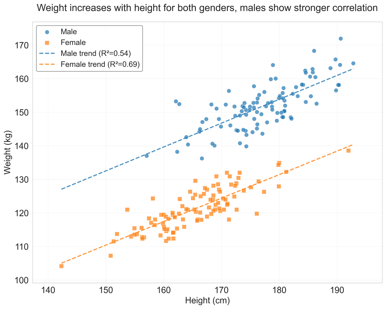
Scatter plot of height vs weight colored by gender with regression line
Statistical•matplotlib, seaborn
From the chart gallery•Correlation analysis between metrics

Scatterplot

Displays values for two variables as points on a Cartesian coordinate system.

Sample code / prompt

import matplotlib.pyplot as plt
import numpy as np
from scipy import stats
import pandas as pd

# Generate sample data
np.random.seed(42)
n_samples = 200
height = np.random.normal(170, 8, n_samples)
weight = height * 0.6 + np.random.normal(0, 8, n_samples) - 50
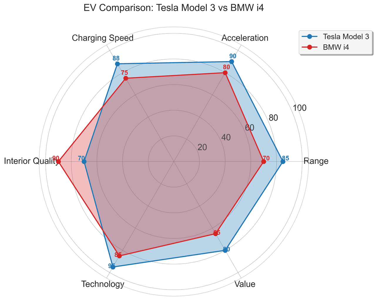
Radar chart comparing performance metrics of two models
Comparison•matplotlib, plotly
From the chart gallery•Product feature comparison

Radar Chart

Displays multivariate data on axes starting from a central point.

Sample code / prompt

import numpy as np
import matplotlib.pyplot as plt
from matplotlib.patches import Circle
import pandas as pd

# EV Model comparison data (0-100 scale)
categories = ['Range', 'Acceleration', 'Charging Speed',
              'Interior Quality', 'Technology', 'Value']
tesla_scores = [85, 90, 88, 70, 95, 80]
bmw_scores = [70, 80, 75, 90, 85, 65]
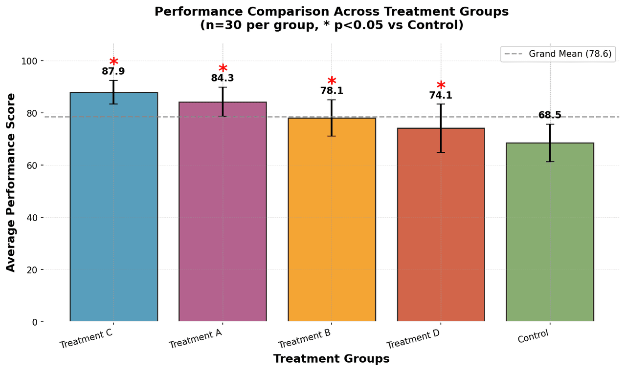
Bar chart comparing average scores across 5 groups with error bars
Comparison•matplotlib, seaborn
From the chart gallery•Comparing performance across categories

Bar Chart

Compares categorical data using rectangular bars with heights proportional to values.

Sample code / prompt

import numpy as np
import pandas as pd
import matplotlib.pyplot as plt
import seaborn as sns
from scipy import stats

# Generate performance scores for 5 treatment groups
np.random.seed(42)
groups = ['Control', 'Treatment A', 'Treatment B', 'Treatment C', 'Treatment D']
n_samples = 30

Run PCA on Your Data in 30 Seconds

Upload a CSV with numeric columns and Plotivy handles the rest - scaling, decomposition, biplots, scree plots, and journal-ready export.