Menu

Time-to-Event Analysis

Kaplan-Meier Survival Curves with Log-Rank Tests

Survival analysis is the cornerstone of clinical trial reporting. Plotivy generates Kaplan-Meier curves with censoring marks, median survival annotations, log-rank p-values, and number-at-risk tables from your data.

Understanding Kaplan-Meier Curves

The Kaplan-Meier estimator is a non-parametric method for estimating the survival function from time-to-event data. It handles censored observations (patients lost to follow-up) and is the standard reporting format required by JAMA, NEJM, and Lancet.

Step function

Drops at each event time - the characteristic staircase shape

Censoring ticks

Vertical marks showing when patients left the study without events

Median survival

Time at which 50% survival probability is reached

Log-rank test

Compares curves between groups - the primary statistical test

Live Code Lab: Kaplan-Meier Curve

This code implements the full KM estimator from scratch, draws step curves for two treatment arms, adds censoring marks, median survival annotations, and a log-rank p-value. Everything is editable.

Live Code Editor
Code EditorPython
Loading editor...
Live Preview

Preparing preview

Running once automatically on first load

Learn by Experimenting

This is a safe playground for learning! Try changing:

  • • Colors: Modify color values to see different palettes
  • • Numbers: Adjust sizes, positions, or data ranges
  • • Labels: Update titles, axis names, or legends

Edit the code, run it, then open the full data visualization tool to continue with your own dataset.

Bonus: Forest Plot (Hazard Ratios)

Forest plots display hazard ratios from Cox regression - the standard companion to KM curves in clinical publications. The reference line at HR=1 separates protective and harmful effects.

Live Code Editor
Code EditorPython
Loading editor...
Live Preview

Preparing preview

Running once automatically on first load

Learn by Experimenting

This is a safe playground for learning! Try changing:

  • • Colors: Modify color values to see different palettes
  • • Numbers: Adjust sizes, positions, or data ranges
  • • Labels: Update titles, axis names, or legends

Edit the code, run it, then open the full data visualization tool to continue with your own dataset.

Survival Analysis Features

Auto KM estimation

Upload time-to-event data and Plotivy computes the KM estimator, handles censoring, and draws step curves automatically.

Built-in log-rank test

Statistical comparison of survival curves with p-value annotation - no manual calculation required.

Number-at-risk table

Generates the risk table below the curve that most clinical journals require for publication.

CONSORT compliance

Figures meet CONSORT reporting guidelines with proper censoring marks, labels, and sizing.

Chart gallery

Related Clinical Charts

More visualization types for clinical research

Browse all chart types →
Box and whisker plot comparing gene expression across 4 genotypes with significance brackets
Distribution•seaborn, matplotlib
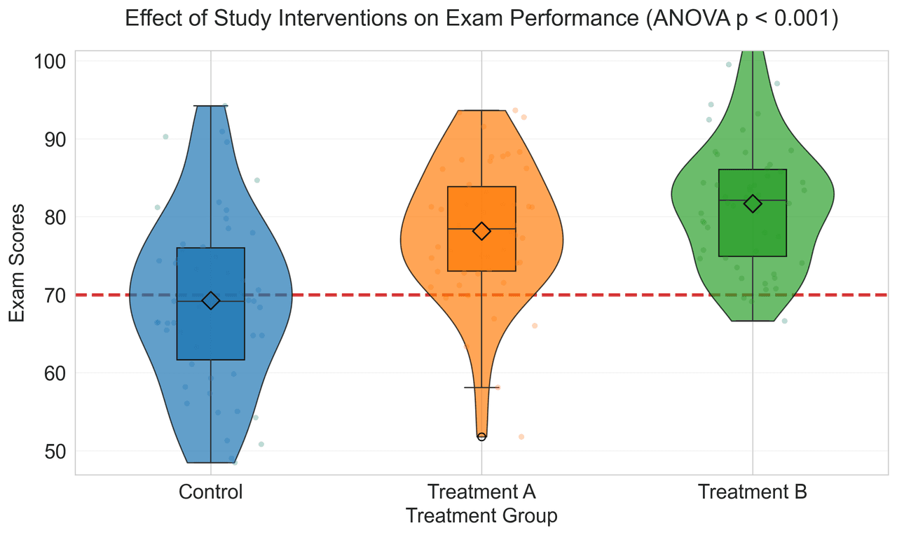
From the chart gallery•Comparing experimental groups in scientific research

Box and Whisker Plot

Displays data distribution using quartiles, median, and outliers in a standardized format.

Sample code / prompt

import numpy as np
import pandas as pd
import matplotlib.pyplot as plt
import seaborn as sns
from scipy import stats

# Generate gene expression data for 4 genotypes
np.random.seed(42)
genotypes = ['WT', 'KO1', 'KO2', 'Mutant']
n_per_group = 20
Violin plot comparing score distributions across 3 groups with inner box plots
Distribution•seaborn, matplotlib
From the chart gallery•Comparing treatment effects across groups

Violin Plot

Combines box plots with kernel density to show distribution shape across groups.

Sample code / prompt

import matplotlib.pyplot as plt
import seaborn as sns
import pandas as pd
import numpy as np
from scipy.stats import f_oneway

# Generate exam score data for 3 groups
np.random.seed(42)
control = np.random.normal(72, 12, 50)
treatment_a = np.random.normal(78, 10, 50)
Scatter plot of height vs weight colored by gender with regression line
Statistical•matplotlib, seaborn
From the chart gallery•Correlation analysis between metrics

Scatterplot

Displays values for two variables as points on a Cartesian coordinate system.

Sample code / prompt

import matplotlib.pyplot as plt
import numpy as np
from scipy import stats
import pandas as pd

# Generate sample data
np.random.seed(42)
n_samples = 200
height = np.random.normal(170, 8, n_samples)
weight = height * 0.6 + np.random.normal(0, 8, n_samples) - 50
Bar chart comparing average scores across 5 groups with error bars
Comparison•matplotlib, seaborn
From the chart gallery•Comparing performance across categories

Bar Chart

Compares categorical data using rectangular bars with heights proportional to values.

Sample code / prompt

import numpy as np
import pandas as pd
import matplotlib.pyplot as plt
import seaborn as sns
from scipy import stats

# Generate performance scores for 5 treatment groups
np.random.seed(42)
groups = ['Control', 'Treatment A', 'Treatment B', 'Treatment C', 'Treatment D']
n_samples = 30
Multi-line graph showing temperature trends for 3 cities over a year
Time Series•matplotlib, seaborn
From the chart gallery•Stock price tracking over time

Line Graph

Displays data points connected by straight line segments to show trends over time.

Sample code / prompt

import matplotlib.pyplot as plt
import numpy as np

# Generate temperature data for 3 major US cities over 12 months
months = ['Jan', 'Feb', 'Mar', 'Apr', 'May', 'Jun', 'Jul', 'Aug', 'Sep', 'Oct', 'Nov', 'Dec']
nyc = [30, 32, 40, 52, 65, 75, 82, 81, 74, 63, 50, 38]
miami = [65, 66, 70, 76, 82, 87, 90, 90, 87, 80, 72, 66]
chicago = [25, 27, 35, 48, 62, 72, 80, 79, 71, 60, 45, 32]

# Create figure with enhanced styling

Your Clinical Data Deserves Better Curves

Upload time-to-event data and get journal-ready Kaplan-Meier curves with log-rank tests and number-at-risk tables in seconds.