Violin Plot

Violin plots combine the summary statistics of box plots with the distribution shape visualization of kernel density estimation. The width of each 'violin' represents the density of data at that value, providing more insight into the distribution shape than box plots alone. They're excellent for comparing distributions across multiple groups, especially when distributions may be multimodal.

Example Visualization

Violin plot comparing score distributions across 3 groups with inner box plots

Try this prompt

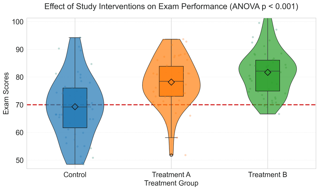
"Create a violin plot comparing 'Exam Scores' across 3 treatment groups: Control, Treatment A, and Treatment B. Generate realistic educational data with 50 students per group. Control: mean=72, sd=12 (normal). Treatment A: mean=78, sd=10 (slight improvement). Treatment B: mean=82, sd=8 (significant improvement, less variance). Include embedded box plots showing quartiles, median line, and mean diamond marker. Add individual data points as a strip plot with jitter (alpha=0.3). Perform and annotate ANOVA p-value. Use distinct colors for each group. Add horizontal reference line at passing score (70). Title: 'Effect of Study Interventions on Exam Performance'."

Generate this now

Python Code Example

Loading code...

Common Use Cases

1Comparing treatment effects across groups
2Salary distribution by department
3Test score analysis by class
4Bimodal distribution detection

Pro Tips

Include inner box plots for summary statistics

Use split violins for two-group comparisons

Scale violin widths consistently or by sample size