ANOVA Visualization in Python with Post-Hoc Significance Brackets
Technique overview
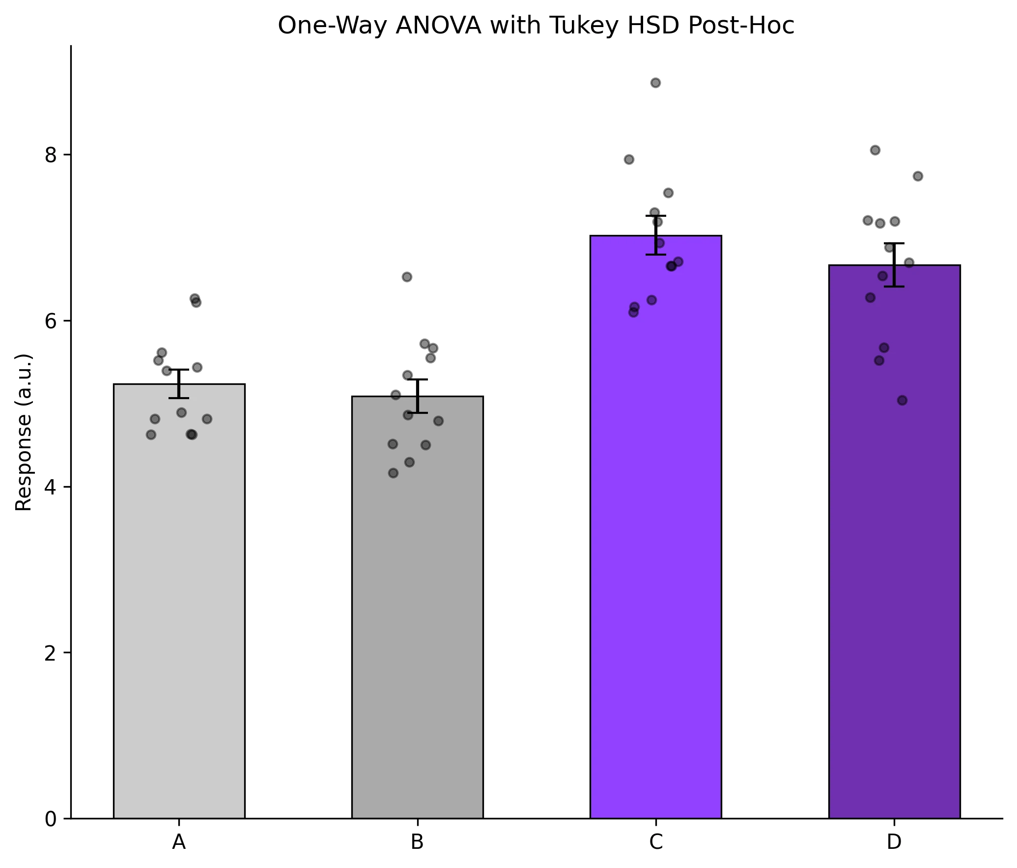
Run one-way ANOVA with Tukey HSD post-hoc and add significance brackets to grouped bar charts. Includes non-parametric Kruskal-Wallis with Dunn test alternative.
When your experiment has three or more groups - different drug concentrations, multiple cell lines, or several time points - you cannot simply run pairwise t-tests without inflating the false-positive rate. One-way ANOVA tests whether any group mean differs significantly from the others, and a post-hoc test (Tukey HSD is the most common) identifies which specific pairs differ. The statistical analysis is straightforward, but the visualization challenge is considerable: you need to draw significance brackets for every significant pair on the same bar chart without overlapping annotations. This page provides the complete ANOVA-to-figure pipeline, handling the bracket geometry automatically for any number of groups.
Key points
- Run one-way ANOVA with Tukey HSD post-hoc and add significance brackets to grouped bar charts. Includes non-parametric Kruskal-Wallis with Dunn test alternative.
- When your experiment has three or more groups - different drug concentrations, multiple cell lines, or several time points - you cannot simply run pairwise t-tests without inflating the false-positive rate.
- One-way ANOVA tests whether any group mean differs significantly from the others, and a post-hoc test (Tukey HSD is the most common) identifies which specific pairs differ.
- The statistical analysis is straightforward, but the visualization challenge is considerable: you need to draw significance brackets for every significant pair on the same bar chart without overlapping annotations.
Example Visualization
Review the example first, then use the live editor below to run and customize the full workflow.
Mathematical Foundation
When your experiment has three or more groups - different drug concentrations, multiple cell lines, or several time points - you cannot simply run pairwise t-tests without inflating the false-positive rate.
Equation
F = MS_between / MS_within = (SS_between / (k-1)) / (SS_within / (N-k))Parameter breakdown
When to use this technique
Use one-way ANOVA when comparing means of 3 or more independent groups under the assumptions of normality and homogeneity of variance. If these assumptions are violated, use the Kruskal-Wallis test as a non-parametric alternative.
Apply This Technique Now
Run this analysis workflow with AI in seconds. Use the prepared technique prompt or bring your own dataset.
View example prompt
"Compare my treatment groups with one-way ANOVA, run Tukey HSD post-hoc, and create a bar chart with error bars and significance brackets showing all significant pairs"
How to apply this technique in 30 seconds
Generate
Run the example prompt and let AI generate this technique automatically.
Refine and Export
Adjust code or prompt, then export publication-ready figures.
Implementation Code
The core data processing logic. Copy this block and replace the sample data with your measurements.
import numpy as np
from scipy import stats
from statsmodels.stats.multicomp import pairwise_tukeyhsd

# --- Experimental data: 4 treatment groups ---
np.random.seed(42)
group_a = np.random.normal(5.0, 0.8, 12)
group_b = np.random.normal(5.5, 0.7, 12)
group_c = np.random.normal(7.2, 0.9, 12)
group_d = np.random.normal(7.0, 1.0, 12)

# --- One-way ANOVA ---
f_stat, p_value = stats.f_oneway(group_a, group_b, group_c, group_d)
print(f"ANOVA: F={f_stat:.3f}, p={p_value:.4e}")

# --- Tukey HSD post-hoc ---
all_data = np.concatenate([group_a, group_b, group_c, group_d])
labels = (['A'] * 12 + ['B'] * 12 + ['C'] * 12 + ['D'] * 12)
tukey = pairwise_tukeyhsd(all_data, labels, alpha=0.05)
print("\nTukey HSD results:")
print(tukey)

# --- Effect size (eta-squared) ---
grand_mean = all_data.mean()
ss_between = sum(len(g) * (g.mean() - grand_mean) ** 2
                 for g in [group_a, group_b, group_c, group_d])
ss_total = np.sum((all_data - grand_mean) ** 2)
eta_sq = ss_between / ss_total
print(f"\nEta-squared: {eta_sq:.3f}")Visualization Code
Complete matplotlib code for a publication-ready figure. Copy, paste into your notebook, and adjust labels to match your data.
import numpy as np
import matplotlib.pyplot as plt
from scipy import stats
from statsmodels.stats.multicomp import pairwise_tukeyhsd

def p_to_stars(p):
    if p < 0.001: return '***'
    if p < 0.01:  return '**'
    if p < 0.05:  return '*'
    return 'ns'

def add_bracket(ax, x1, x2, y, h, text):
    ax.plot([x1, x1, x2, x2], [y, y + h, y + h, y], lw=1.2, color='black')
    ax.text((x1 + x2) / 2, y + h, text, ha='center', va='bottom', fontsize=10)

np.random.seed(42)
groups = {
    'A': np.random.normal(5.0, 0.8, 12),
    'B': np.random.normal(5.5, 0.7, 12),
    'C': np.random.normal(7.2, 0.9, 12),
    'D': np.random.normal(7.0, 1.0, 12),
}
names = list(groups.keys())
means = [g.mean() for g in groups.values()]
sems  = [stats.sem(g) for g in groups.values()]

# Tukey HSD
all_data = np.concatenate(list(groups.values()))
labels = sum([[n] * 12 for n in names], [])
tukey = pairwise_tukeyhsd(all_data, labels, alpha=0.05)

fig, ax = plt.subplots(figsize=(7, 6))
x_pos = np.arange(len(names))
colors_bar = ['#cccccc', '#aaaaaa', '#9240ff', '#7030b0']
ax.bar(x_pos, means, yerr=sems, width=0.55, capsize=5,
       color=colors_bar, edgecolor='black', lw=0.8)

for i, (name, data) in enumerate(groups.items()):
    jitter = np.random.uniform(-0.12, 0.12, size=len(data))
    ax.scatter(np.full_like(data, i) + jitter, data, s=18,
               color='black', alpha=0.45, zorder=5)

# Significance brackets for significant pairs
y_max = max(m + s for m, s in zip(means, sems)) + 0.4
step = 0.45
sig_pairs = [(r[0], r[1], r[3]) for r in tukey._results_table.data[1:]
             if r[5] == True]  # reject = True
for idx, (g1, g2, pval) in enumerate(sig_pairs):
    x1, x2 = names.index(g1), names.index(g2)
    y = y_max + idx * step
    add_bracket(ax, x1, x2, y, 0.15, p_to_stars(pval))

ax.set_xticks(x_pos)
ax.set_xticklabels(names)
ax.set_ylabel('Response (a.u.)')
ax.set_title('One-Way ANOVA with Tukey HSD Post-Hoc', fontsize=12)
ax.spines[['top', 'right']].set_visible(False)
plt.tight_layout()
plt.savefig('anova_brackets.png', dpi=300, bbox_inches='tight')
plt.show()Kruskal-Wallis with Dunn Post-Hoc (Non-Parametric)
When your data violate ANOVA assumptions - non-normal distributions, ordinal data, or small sample sizes with skewness - the Kruskal-Wallis H-test is the appropriate non-parametric alternative. For pairwise post-hoc comparisons, use the Dunn test with Bonferroni correction.
import numpy as np
import matplotlib.pyplot as plt
from scipy import stats
import scikit_posthocs as sp

np.random.seed(42)
groups = {
    'Control':  np.random.exponential(2.0, 12) + 3,
    'Low':      np.random.exponential(2.5, 12) + 4,
    'Medium':   np.random.exponential(3.0, 12) + 6,
    'High':     np.random.exponential(3.5, 12) + 8,
}

# --- Kruskal-Wallis ---
h_stat, p_kw = stats.kruskal(*groups.values())
print(f"Kruskal-Wallis: H={h_stat:.3f}, p={p_kw:.4e}")

# --- Dunn post-hoc ---
all_data = np.concatenate(list(groups.values()))
labels = sum([[k] * len(v) for k, v in groups.items()], [])
dunn = sp.posthoc_dunn([groups[k] for k in groups], p_adjust='bonferroni')
print("\nDunn test p-values:")
print(dunn)

# --- Plot ---
fig, ax = plt.subplots(figsize=(7, 5))
positions = range(len(groups))
bp = ax.boxplot(groups.values(), positions=positions, patch_artist=True,
                widths=0.4, showfliers=False)
colors_box = ['#cccccc', '#aaaaaa', '#9240ff', '#7030b0']
for patch, color in zip(bp['boxes'], colors_box):
    patch.set_facecolor(color)
    patch.set_alpha(0.7)

for i, (name, data) in enumerate(groups.items()):
    jitter = np.random.uniform(-0.08, 0.08, size=len(data))
    ax.scatter(np.full_like(data, i) + jitter, data, s=18,
               color='black', alpha=0.4, zorder=5)

ax.set_xticks(positions)
ax.set_xticklabels(groups.keys())
ax.set_ylabel('Response')
ax.set_title(f'Kruskal-Wallis H-test (p = {p_kw:.4f})', fontsize=12)
ax.spines[['top', 'right']].set_visible(False)
plt.tight_layout()
plt.savefig('kruskal_wallis.png', dpi=300, bbox_inches='tight')
plt.show()Common Errors and How to Fix Them
Unequal group sizes causing Type I error inflation
Why: Classical ANOVA is robust to mild imbalance, but large differences in group sizes combined with unequal variances can inflate false positive rates.
Fix: Use Welch's ANOVA (scipy does not have it built-in, but pingouin.welch_anova does) or the Kruskal-Wallis test when group sizes differ substantially.
Residuals are not normally distributed
Why: ANOVA assumes normal residuals. Skewed distributions, outliers, or count data can violate this.
Fix: Run a Shapiro-Wilk test on residuals. If non-normal, transform the data (log, sqrt) or switch to Kruskal-Wallis.
Heteroscedasticity (unequal variances across groups)
Why: Groups with larger means often have larger variances (e.g., Poisson-like data). This violates ANOVA's homogeneity-of-variance assumption.
Fix: Run Levene's test. If significant, use Welch's ANOVA or transform the data. Do not proceed with standard ANOVA when variances are clearly unequal.
Running ANOVA without post-hoc tests
Why: ANOVA only tells you that at least one group differs. Without a post-hoc test, you cannot determine which pairs are significant.
Fix: Always follow a significant ANOVA result with Tukey HSD (balanced groups) or Games-Howell (unequal variances) to identify specific pairs.
Too many groups reduce statistical power
Why: With many groups and a fixed total N, each group has fewer observations, and the multiple-comparison correction becomes increasingly stringent.
Fix: Plan the experiment with a power analysis. If you have 6+ groups, consider pre-specified contrasts instead of all-pairwise comparisons.
Frequently Asked Questions
Apply ANOVA Visualization in Python with Post-Hoc Significance Brackets to Your Data
Upload your dataset and Plotivy generates the Python code, runs the analysis, and produces a publication-ready figure.
Generate Code for This TechniquePython Libraries
Quick Info
- Domain
- Statistics
- Typical Audience
- Biology PhD students comparing three or more treatment groups who need correct post-hoc testing with publication-ready significance annotations