Dose-Response Curve Fitting in Python (Hill Equation, EC50/IC50)
Technique overview
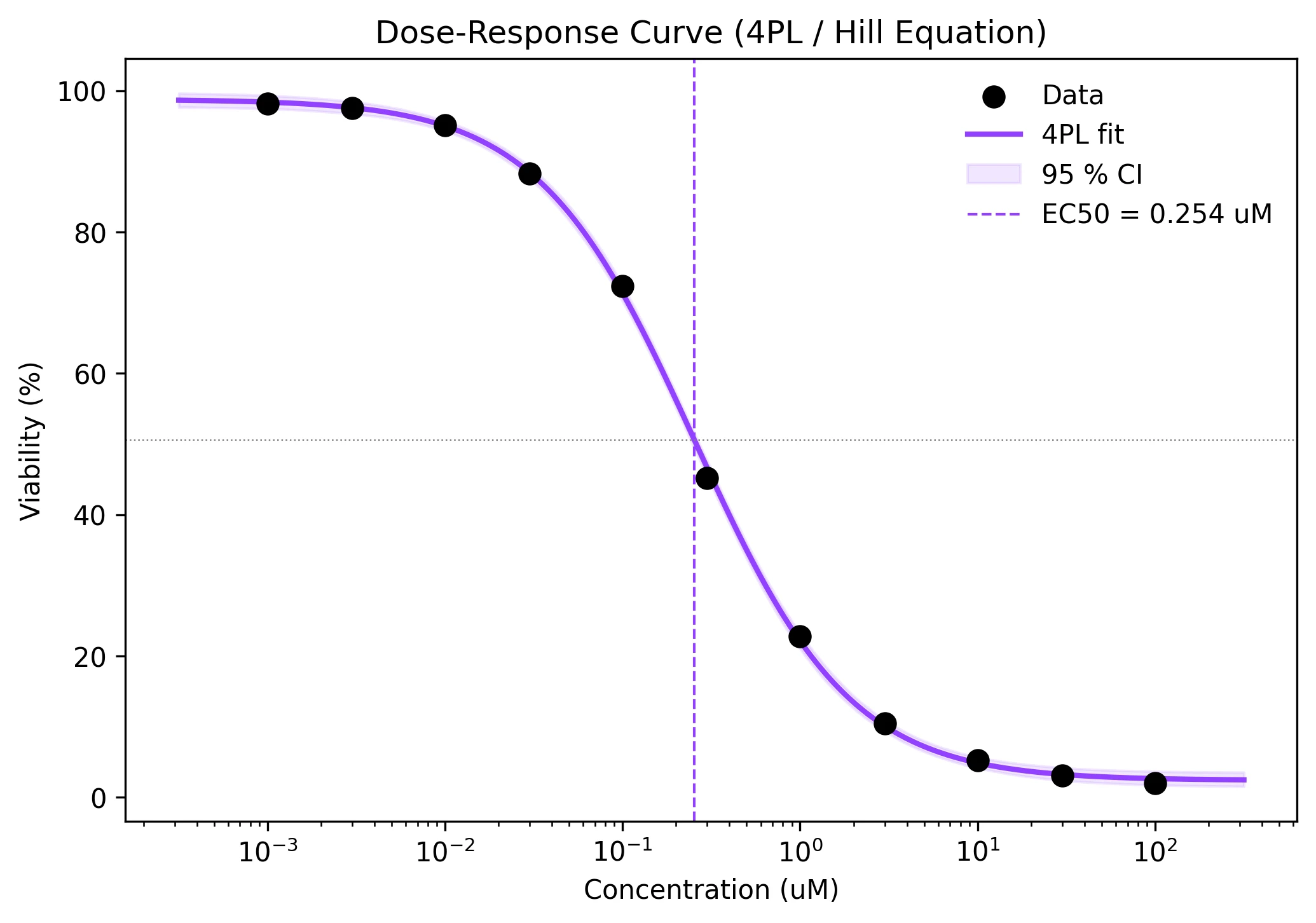
Fit dose-response data using the Hill equation and 4PL model. Extract EC50/IC50 with confidence intervals and produce publication-ready sigmoidal curves.
Dose-response analysis is central to pharmacology, toxicology, and drug discovery. Whether you are determining the IC50 of a kinase inhibitor from a cell viability assay, calculating the EC50 of an agonist from a cAMP reporter, or establishing a lethal dose for an environmental contaminant, the 4-parameter logistic (4PL) model - also known as the Hill equation - is the standard curve to fit. The non-trivial part is handling the log-scale x-axis, providing good initial guesses so the optimizer converges, and extracting EC50/IC50 with proper confidence intervals rather than just point estimates. This page provides the end-to-end Python code.
Key points
- Fit dose-response data using the Hill equation and 4PL model. Extract EC50/IC50 with confidence intervals and produce publication-ready sigmoidal curves.
- Dose-response analysis is central to pharmacology, toxicology, and drug discovery.
- Whether you are determining the IC50 of a kinase inhibitor from a cell viability assay, calculating the EC50 of an agonist from a cAMP reporter, or establishing a lethal dose for an environmental contaminant, the 4-parameter logistic (4PL) model - also known as the Hill equation - is the standard curve to fit.
- The non-trivial part is handling the log-scale x-axis, providing good initial guesses so the optimizer converges, and extracting EC50/IC50 with proper confidence intervals rather than just point estimates.
Example Visualization
Review the example first, then use the live editor below to run and customize the full workflow.
Mathematical Foundation
Dose-response analysis is central to pharmacology, toxicology, and drug discovery.
Equation
f(x) = Bottom + (Top - Bottom) / (1 + (x / EC50)^n)Parameter breakdown
When to use this technique
Use the 4PL/Hill model when your dose-response data follows a sigmoidal shape on a log-concentration scale. Ensure you have data points spanning both plateaus (top and bottom) and the transition region. If the curve does not reach both plateaus, the fit may be poorly constrained.
Apply This Technique Now
Run this analysis workflow with AI in seconds. Use the prepared technique prompt or bring your own dataset.
View example prompt
"Fit a 4-parameter logistic dose-response curve to my data, extract EC50 with 95% confidence interval, and plot on log-x scale with data points and best-fit line"
How to apply this technique in 30 seconds
Generate
Run the example prompt and let AI generate this technique automatically.
Refine and Export
Adjust code or prompt, then export publication-ready figures.
Implementation Code
The core data processing logic. Copy this block and replace the sample data with your measurements.
import numpy as np
from scipy.optimize import curve_fit

def hill_equation(x, bottom, top, ec50, n):
    return bottom + (top - bottom) / (1 + (x / ec50) ** n)

# --- Dose-response data (e.g., cell viability assay) ---
concentrations = np.array([0.001, 0.003, 0.01, 0.03, 0.1, 0.3, 1.0,
                           3.0, 10.0, 30.0, 100.0])  # uM
responses = np.array([98.2, 97.5, 95.1, 88.3, 72.4, 45.2, 22.8,
                      10.5, 5.3, 3.1, 2.0])  # % viability

# --- Initial guesses ---
p0 = [responses.min(), responses.max(),
      concentrations[len(concentrations) // 2], 1.0]

# --- Fit with bounds to prevent negative EC50 ---
bounds = ([0, 0, 1e-6, 0.1], [200, 200, 1e4, 10])
popt, pcov = curve_fit(hill_equation, concentrations, responses,
                       p0=p0, bounds=bounds, maxfev=10000)
perr = np.sqrt(np.diag(pcov))

labels = ['Bottom', 'Top', 'EC50', 'Hill n']
for name, val, err in zip(labels, popt, perr):
print(f"{name:8s}: {val:.4f} +/- {err:.4f}")Visualization Code
Complete matplotlib code for a publication-ready figure. Copy, paste into your notebook, and adjust labels to match your data.
import numpy as np
import matplotlib.pyplot as plt
from scipy.optimize import curve_fit

def hill_equation(x, bottom, top, ec50, n):
    return bottom + (top - bottom) / (1 + (x / ec50) ** n)

conc = np.array([0.001, 0.003, 0.01, 0.03, 0.1, 0.3, 1.0,
                 3.0, 10.0, 30.0, 100.0])
resp = np.array([98.2, 97.5, 95.1, 88.3, 72.4, 45.2, 22.8,
                 10.5, 5.3, 3.1, 2.0])

p0 = [resp.min(), resp.max(), conc[len(conc)//2], 1.0]
bounds = ([0, 0, 1e-6, 0.1], [200, 200, 1e4, 10])
popt, pcov = curve_fit(hill_equation, conc, resp, p0=p0,
                       bounds=bounds, maxfev=10000)

x_fit = np.logspace(np.log10(conc.min()) - 0.5,
                    np.log10(conc.max()) + 0.5, 300)
y_fit = hill_equation(x_fit, *popt)

# --- Bootstrap CI ---
n_boot = 500
y_boot = np.zeros((n_boot, len(x_fit)))
for i in range(n_boot):
    p_sample = np.random.multivariate_normal(popt, pcov)
    p_sample[2] = max(p_sample[2], 1e-6)
    y_boot[i] = hill_equation(x_fit, *p_sample)
ci_lo = np.percentile(y_boot, 2.5, axis=0)
ci_hi = np.percentile(y_boot, 97.5, axis=0)

fig, ax = plt.subplots(figsize=(7, 5))
ax.scatter(conc, resp, s=60, color='black', zorder=5, label='Data')
ax.plot(x_fit, y_fit, color='#9240ff', lw=2, label='4PL fit')
ax.fill_between(x_fit, ci_lo, ci_hi, color='#9240ff', alpha=0.12,
                label='95 % CI')
ax.axvline(popt[2], color='#9240ff', ls='--', lw=1,
           label=f'EC50 = {popt[2]:.3f} uM')
ax.axhline((popt[0]+popt[1])/2, color='gray', ls=':', lw=0.6)
ax.set_xscale('log')
ax.set_xlabel('Concentration (uM)')
ax.set_ylabel('Viability (%)')
ax.set_title('Dose-Response Curve (4PL / Hill Equation)', fontsize=12)
ax.legend(frameon=False)
plt.tight_layout()
plt.savefig('dose_response.png', dpi=300, bbox_inches='tight')
plt.show()Multi-Compound Comparison on a Single Plot
In drug screening, you often need to compare dose-response curves for multiple compounds side by side. Plotting them on the same axes with shared x-scale makes it easy to visually compare EC50 values, Hill slopes, and maximal efficacy. This code fits each compound independently and overlays the results.
import numpy as np
import matplotlib.pyplot as plt
from scipy.optimize import curve_fit

def hill_equation(x, bottom, top, ec50, n):
    return bottom + (top - bottom) / (1 + (x / ec50) ** n)

conc = np.array([0.001, 0.003, 0.01, 0.03, 0.1, 0.3, 1.0,
                 3.0, 10.0, 30.0, 100.0])
compounds = {
    'Compound A': np.array([99, 97, 94, 85, 65, 38, 18, 8, 4, 2.5, 2]),
    'Compound B': np.array([98, 96, 92, 80, 55, 30, 15, 9, 6, 5, 4.5]),
    'Compound C': np.array([100, 99, 97, 93, 82, 60, 35, 15, 6, 3, 2]),
}
colors = ['#9240ff', '#e67e22', '#27ae60']
bounds = ([0, 0, 1e-6, 0.1], [200, 200, 1e4, 10])

fig, ax = plt.subplots(figsize=(8, 5))
x_fit = np.logspace(-3.5, 2.5, 300)

for (name, resp), color in zip(compounds.items(), colors):
    p0 = [resp.min(), resp.max(), conc[len(conc)//2], 1.0]
    popt, _ = curve_fit(hill_equation, conc, resp, p0=p0,
                        bounds=bounds, maxfev=10000)
    y_fit = hill_equation(x_fit, *popt)
    ax.scatter(conc, resp, s=40, color=color, zorder=5)
    ax.plot(x_fit, y_fit, color=color, lw=2,
            label=f'{name} (EC50={popt[2]:.3f})')

ax.set_xscale('log')
ax.set_xlabel('Concentration (uM)')
ax.set_ylabel('Viability (%)')
ax.set_title('Multi-Compound Dose-Response Comparison', fontsize=12)
ax.legend(frameon=False, fontsize=9)
ax.spines[['top', 'right']].set_visible(False)
plt.tight_layout()
plt.savefig('multi_compound.png', dpi=300, bbox_inches='tight')
plt.show()Common Errors and How to Fix Them
Fit does not converge for steep Hill slopes (n > 5)
Why: Very steep curves (step-like transitions) create sharp gradients in parameter space where the optimizer struggles to find a stable minimum.
Fix: Provide a tight initial guess for n (e.g., 2-3) and use bounds such as n in [0.1, 10]. If the data truly has a step-like transition, consider a logistic regression approach.
RuntimeWarning: divide by zero in log when plotting
Why: Concentrations of exactly 0.0 cannot be plotted on a logarithmic x-axis.
Fix: Remove the zero-concentration control before curve fitting, or replace it with a very small positive value (e.g., 1e-10) for plotting purposes only. Use the zero data point for the "Top" initial guess.
Normalisation error: response percentages exceed 100 % or go below 0 %
Why: Raw assay data may not be properly normalized to controls, leading to out-of-range values that confuse the optimizer.
Fix: Normalize: response_pct = (raw - negative_ctrl) / (positive_ctrl - negative_ctrl) * 100. Clip to [0, 100] if measurement noise causes minor exceedances.
Insufficient concentration range - fit does not reach both plateaus
Why: If the data does not include concentrations well above and below EC50, the Bottom and Top parameters are unconstrained.
Fix: Extend the dilution series by at least 2 log units in each direction from the expected EC50. Alternatively, fix Top to 100 and Bottom to 0 if you have normalized data and are confident about the plateaus.
Cannot fit if EC50 initial guess is way off
Why: The Hill equation is highly sensitive to the EC50 starting value. A poor guess can lead to convergence at a local minimum.
Fix: Estimate EC50 from the data: find the concentration at which the response is closest to the midpoint of your data range. Use that as p0 for EC50.
Frequently Asked Questions
Python Statistics Code Templates for Biologists
Get 10 complete, runnable Python code snippets for the most common biological statistical tests, each with explanations and publication-ready figure output. Stop fighting with matplotlib!
Python Libraries
Quick Info
- Domain
- Biological
- Typical Audience
- Pharmacologists, cell biologists, and toxicologists analyzing drug response data who need EC50/IC50 values with proper statistical uncertainties