Michaelis-Menten Fitting in Python for Enzyme Kinetics
Technique overview
Fit Michaelis-Menten enzyme kinetics data to extract Km and Vmax with uncertainties. Includes Lineweaver-Burk plots and Hill equation extension.
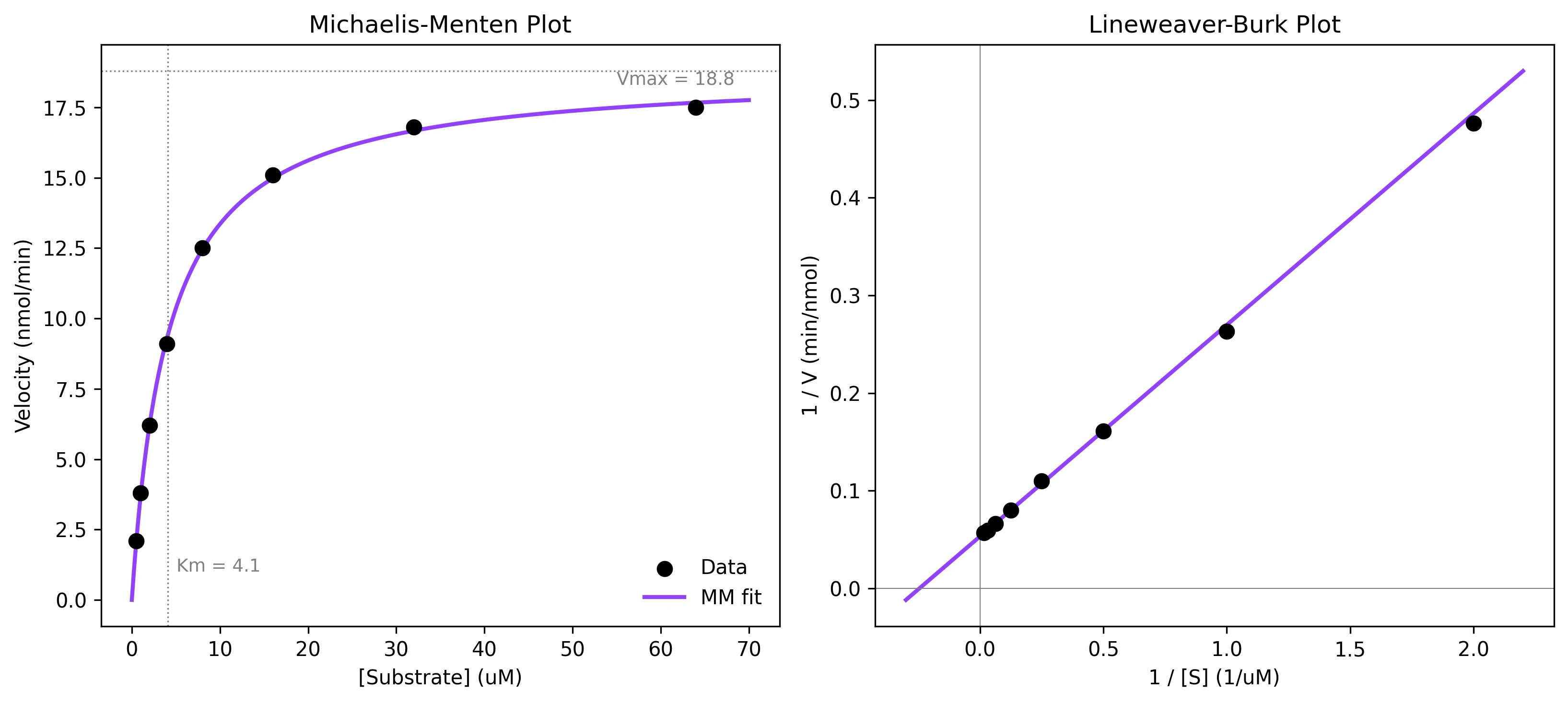
Michaelis-Menten kinetics is the cornerstone of enzymology. Every time you characterize a new enzyme construct, evaluate the effect of a mutation on catalytic efficiency, or screen inhibitors by measuring shifts in apparent Km, you need to fit the hyperbolic rate equation to your substrate-velocity data and extract Km and Vmax with proper uncertainties. While the Lineweaver-Burk double-reciprocal plot was historically used because it linearises the equation, modern practice uses direct nonlinear regression because it avoids the statistical distortions introduced by reciprocal transformation. This page covers both approaches - nonlinear fitting as the primary method and Lineweaver-Burk as a diagnostic companion plot.
Key points
- Fit Michaelis-Menten enzyme kinetics data to extract Km and Vmax with uncertainties. Includes Lineweaver-Burk plots and Hill equation extension.
- Michaelis-Menten kinetics is the cornerstone of enzymology.
- Every time you characterize a new enzyme construct, evaluate the effect of a mutation on catalytic efficiency, or screen inhibitors by measuring shifts in apparent Km, you need to fit the hyperbolic rate equation to your substrate-velocity data and extract Km and Vmax with proper uncertainties.
- While the Lineweaver-Burk double-reciprocal plot was historically used because it linearises the equation, modern practice uses direct nonlinear regression because it avoids the statistical distortions introduced by reciprocal transformation.
Example Visualization
Review the example first, then use the live editor below to run and customize the full workflow.
Mathematical Foundation
Michaelis-Menten kinetics is the cornerstone of enzymology.
Equation
V = Vmax * [S] / (Km + [S])Parameter breakdown
When to use this technique
Use the Michaelis-Menten model for single-substrate enzyme kinetics under steady-state conditions. The substrate concentration range should span from well below Km to well above Km (ideally 0.2 Km to 5 Km). If the plot shows sigmoidal behaviour, consider the Hill equation for cooperative enzymes.
Apply This Technique Now
Run this analysis workflow with AI in seconds. Use the prepared technique prompt or bring your own dataset.
View example prompt
"Fit Michaelis-Menten kinetics to my enzyme data, extract Km and Vmax with uncertainties, and show both the direct plot and Lineweaver-Burk double-reciprocal plot side by side"
How to apply this technique in 30 seconds
Generate
Run the example prompt and let AI generate this technique automatically.
Refine and Export
Adjust code or prompt, then export publication-ready figures.
Implementation Code
The core data processing logic. Copy this block and replace the sample data with your measurements.
import numpy as np
from scipy.optimize import curve_fit

def michaelis_menten(S, Vmax, Km):
    return Vmax * S / (Km + S)

# --- Enzyme kinetics assay data ---
substrate_conc = np.array([0.5, 1.0, 2.0, 4.0, 8.0, 16.0, 32.0, 64.0])  # uM
velocity = np.array([2.1, 3.8, 6.2, 9.1, 12.5, 15.1, 16.8, 17.5])  # nmol/min

# --- Initial guesses from the data ---
Vmax_guess = velocity.max() * 1.1
Km_guess = substrate_conc[np.argmin(np.abs(velocity - velocity.max()/2))]

popt, pcov = curve_fit(michaelis_menten, substrate_conc, velocity,
                       p0=[Vmax_guess, Km_guess],
                       bounds=([0, 0], [np.inf, np.inf]))
perr = np.sqrt(np.diag(pcov))

print(f"Vmax : {popt[0]:.2f} +/- {perr[0]:.2f} nmol/min")
print(f"Km   : {popt[1]:.2f} +/- {perr[1]:.2f} uM")
print(f"Vmax/Km (catalytic efficiency): {popt[0]/popt[1]:.3f} nmol/min/uM")Visualization Code
Complete matplotlib code for a publication-ready figure. Copy, paste into your notebook, and adjust labels to match your data.
import numpy as np
import matplotlib.pyplot as plt
from scipy.optimize import curve_fit

def michaelis_menten(S, Vmax, Km):
    return Vmax * S / (Km + S)

S = np.array([0.5, 1.0, 2.0, 4.0, 8.0, 16.0, 32.0, 64.0])
V = np.array([2.1, 3.8, 6.2, 9.1, 12.5, 15.1, 16.8, 17.5])

popt, pcov = curve_fit(michaelis_menten, S, V, p0=[18, 4],
                       bounds=([0, 0], [np.inf, np.inf]))
Vmax_fit, Km_fit = popt
perr = np.sqrt(np.diag(pcov))

S_fit = np.linspace(0, 70, 300)
V_fit = michaelis_menten(S_fit, *popt)

fig, (ax1, ax2) = plt.subplots(1, 2, figsize=(11, 5))

# --- Direct plot ---
ax1.scatter(S, V, s=50, color='black', zorder=5, label='Data')
ax1.plot(S_fit, V_fit, color='#9240ff', lw=2, label='MM fit')
ax1.axhline(Vmax_fit, color='gray', ls=':', lw=0.8)
ax1.axvline(Km_fit, color='gray', ls=':', lw=0.8)
ax1.annotate(f'Vmax = {Vmax_fit:.1f}', xy=(55, Vmax_fit - 0.5),
             fontsize=9, color='gray')
ax1.annotate(f'Km = {Km_fit:.1f}', xy=(Km_fit + 1, 1),
             fontsize=9, color='gray')
ax1.set_xlabel('[Substrate] (uM)')
ax1.set_ylabel('Velocity (nmol/min)')
ax1.set_title('Michaelis-Menten Plot', fontsize=12)
ax1.legend(frameon=False)

# --- Lineweaver-Burk ---
inv_S = 1.0 / S
inv_V = 1.0 / V
ax2.scatter(inv_S, inv_V, s=50, color='black', zorder=5)
x_lb = np.linspace(-0.3, inv_S.max() * 1.1, 200)
y_lb = (Km_fit / Vmax_fit) * x_lb + 1.0 / Vmax_fit
ax2.plot(x_lb, y_lb, color='#9240ff', lw=2)
ax2.axhline(0, color='gray', lw=0.5)
ax2.axvline(0, color='gray', lw=0.5)
ax2.set_xlabel('1 / [S] (1/uM)')
ax2.set_ylabel('1 / V (min/nmol)')
ax2.set_title('Lineweaver-Burk Plot', fontsize=12)

plt.tight_layout()
plt.savefig('michaelis_menten.png', dpi=300, bbox_inches='tight')
plt.show()Hill Equation for Cooperative Enzymes
When an enzyme shows cooperativity - the binding of one substrate molecule influences the binding of subsequent molecules - the saturation curve becomes sigmoidal rather than hyperbolic. The Hill equation extends Michaelis-Menten kinetics with a cooperativity coefficient n (Hill coefficient): n > 1 indicates positive cooperativity, n = 1 is non-cooperative (standard MM), and n < 1 indicates negative cooperativity.
import numpy as np
import matplotlib.pyplot as plt
from scipy.optimize import curve_fit

def hill_kinetics(S, Vmax, K_half, n):
    return Vmax * S ** n / (K_half ** n + S ** n)

# --- Cooperative enzyme data (hemoglobin-like sigmoidal curve) ---
S = np.array([0.5, 1.0, 2.0, 4.0, 8.0, 12.0, 16.0, 24.0, 32.0, 48.0, 64.0])
V = np.array([0.3, 0.9, 2.8, 7.5, 13.0, 15.8, 17.0, 17.8, 18.0, 18.2, 18.3])

popt_mm, _ = curve_fit(lambda s, vm, km: vm * s / (km + s), S, V,
                       p0=[18, 5], bounds=([0, 0], [np.inf, np.inf]))
popt_hill, pcov_hill = curve_fit(hill_kinetics, S, V, p0=[18, 5, 2],
                                  bounds=([0, 0, 0.1], [np.inf, np.inf, 10]))
perr = np.sqrt(np.diag(pcov_hill))

S_fit = np.linspace(0, 70, 300)
fig, ax = plt.subplots(figsize=(7, 5))
ax.scatter(S, V, s=50, color='black', zorder=5, label='Data')
ax.plot(S_fit, popt_mm[0] * S_fit / (popt_mm[1] + S_fit),
        color='gray', lw=1.5, ls='--', label=f'MM (Km={popt_mm[1]:.1f})')
ax.plot(S_fit, hill_kinetics(S_fit, *popt_hill), color='#9240ff', lw=2,
        label=f'Hill (n={popt_hill[2]:.2f}, K_half={popt_hill[1]:.1f})')
ax.set_xlabel('[Substrate] (uM)')
ax.set_ylabel('Velocity (nmol/min)')
ax.set_title('Hill Equation: Cooperative Enzyme Kinetics', fontsize=12)
ax.legend(frameon=False)
ax.spines[['top', 'right']].set_visible(False)

print(f"Vmax   : {popt_hill[0]:.2f} +/- {perr[0]:.2f}")
print(f"K_half : {popt_hill[1]:.2f} +/- {perr[1]:.2f}")
print(f"Hill n : {popt_hill[2]:.2f} +/- {perr[2]:.2f}")
plt.tight_layout()
plt.savefig('hill_kinetics.png', dpi=300, bbox_inches='tight')
plt.show()Common Errors and How to Fix Them
Substrate inhibition produces a velocity decrease at high [S]
Why: At very high substrate concentrations, some enzymes exhibit substrate inhibition, causing the velocity to decrease instead of plateauing.
Fix: Use a substrate inhibition model: V = Vmax * S / (Km + S + S^2/Ki). Add Ki as a fourth parameter and include data at high [S].
Km is negative or unreasonably small
Why: Poor initial guesses or insufficient data at low substrate concentrations can cause the optimizer to converge at a non-physical Km value.
Fix: Set bounds=([0, 0], [np.inf, np.inf]) to enforce positive Km and Vmax. Ensure you have data points below, near, and above the expected Km.
Poor initial guess leads to a flat line or wrong asymptote
Why: If Vmax_guess is too low or Km_guess is far off, curve_fit may converge at a local minimum.
Fix: Estimate Vmax from the highest measured velocity (multiply by 1.1 as a safety factor). Estimate Km as the [S] where V is approximately Vmax/2.
Insufficient substrate concentration range
Why: If all data points are far below Km or far above Km, the fit cannot distinguish Vmax and Km independently.
Fix: Span at least 0.2 * Km to 5 * Km. If you do not know Km in advance, perform a pilot experiment with a wide concentration range.
Ignoring cooperativity when the curve is sigmoidal
Why: Fitting a standard Michaelis-Menten model to cooperative data will give biased Km and Vmax estimates.
Fix: Inspect the residuals of the MM fit. If they show systematic curvature, switch to the Hill equation and fit n as a free parameter.
Frequently Asked Questions
Python Statistics Code Templates for Biologists
Get 10 complete, runnable Python code snippets for the most common biological statistical tests, each with explanations and publication-ready figure output. Stop fighting with matplotlib!
Python Libraries
Quick Info
- Domain
- Biological
- Typical Audience
- Biochemistry and enzymology researchers analyzing enzyme kinetics assay data who need Km/Vmax values with proper error propagation