Curve FittingLive Code Editor

160 researchers ran this analysis this month

Gaussian Curve Fitting in Python

Technique overview

Fit Gaussian peaks to spectroscopy, chromatography, or any bell-shaped data using scipy.optimize.curve_fit. Extract peak center, amplitude, and width with uncertainties.

Gaussian curve fitting is one of the most frequently encountered tasks in experimental science. Whether you are extracting emission line widths from a fluorescence spectrum, quantifying a chromatographic peak eluting from an HPLC column, or characterizing the point-spread function of an optical system, the underlying workflow is the same: define a Gaussian model, supply reasonable initial guesses, and let a nonlinear least-squares optimizer converge on the best-fit parameters. This page walks through the entire pipeline in Python using scipy.optimize.curve_fit, from raw data ingestion to publication-ready residual plots, so you can spend less time on boilerplate and more time interpreting your results.

Key points

Fit Gaussian peaks to spectroscopy, chromatography, or any bell-shaped data using scipy.optimize.curve_fit. Extract peak center, amplitude, and width with uncertainties.
Gaussian curve fitting is one of the most frequently encountered tasks in experimental science.
Whether you are extracting emission line widths from a fluorescence spectrum, quantifying a chromatographic peak eluting from an HPLC column, or characterizing the point-spread function of an optical system, the underlying workflow is the same: define a Gaussian model, supply reasonable initial guesses, and let a nonlinear least-squares optimizer converge on the best-fit parameters.
This page walks through the entire pipeline in Python using scipy.optimize.curve_fit, from raw data ingestion to publication-ready residual plots, so you can spend less time on boilerplate and more time interpreting your results.

scipynumpymatplotlib

Example Visualization

Open full screen

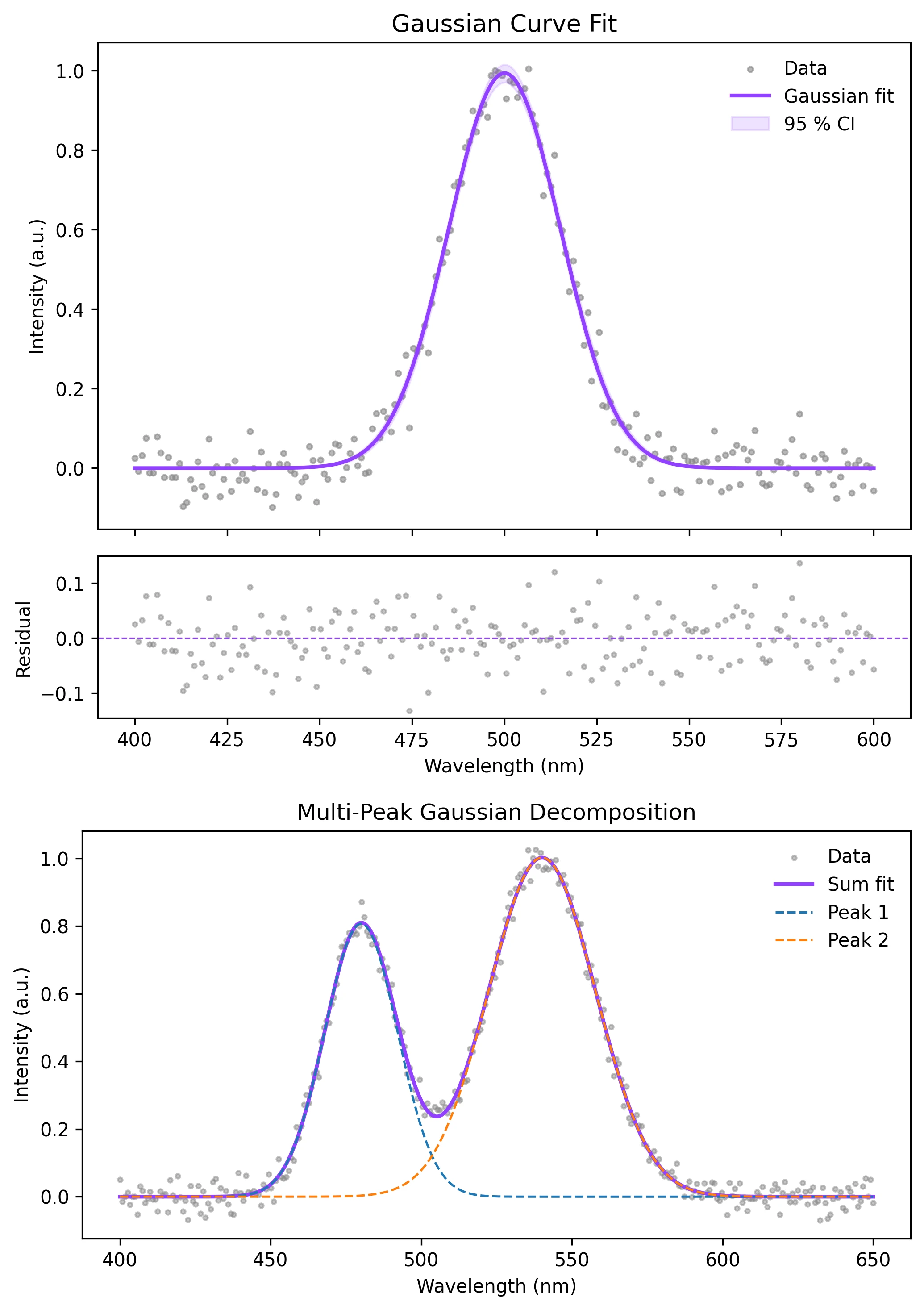
Review the example first, then use the live editor below to run and customize the full workflow.

Mathematical Foundation

Gaussian curve fitting is one of the most frequently encountered tasks in experimental science.

Equation

f(x) = A * exp( -(x - mu)^2 / (2 * sigma^2) )

Parameter breakdown

APeak amplitude (maximum height of the Gaussian)

muPeak center position (mean of the distribution)

sigmaStandard deviation (controls the width; FWHM = 2.355 * sigma)

When to use this technique

Use a single Gaussian fit when your data contains one symmetric, bell-shaped peak riding on a flat or slowly varying baseline. If you see asymmetry or multiple overlapping peaks, consider a multi-peak model or a Voigt profile instead.

Apply This Technique Now

Run this analysis workflow with AI in seconds. Use the prepared technique prompt or bring your own dataset.

Try Technique Prompt Use Your Own Data

View example prompt

Example AI Prompt

"Fit a Gaussian to my spectroscopy data and plot the result with residuals and parameter annotations in Nature style"

How to apply this technique in 30 seconds

Upload Data

Upload your CSV or Excel file in Analyze and keep your column names as-is.

Generate

Run the example prompt and let AI generate this technique automatically.

Refine and Export

Adjust code or prompt, then export publication-ready figures.

Implementation Code

The core data processing logic. Copy this block and replace the sample data with your measurements.

import numpy as np
from scipy.optimize import curve_fit

# --- Define the Gaussian model ---
def gaussian(x, amplitude, center, sigma):
    return amplitude * np.exp(-(x - center) ** 2 / (2 * sigma ** 2))

# --- Simulated spectroscopy data (replace with your own) ---
np.random.seed(42)
x_data = np.linspace(400, 600, 200)
y_true = gaussian(x_data, amplitude=1.0, center=500, sigma=15)
y_data = y_true + np.random.normal(0, 0.05, size=x_data.shape)

# --- Initial parameter guesses ---
p0 = [y_data.max(), x_data[np.argmax(y_data)], 10.0]

# --- Fit ---
popt, pcov = curve_fit(gaussian, x_data, y_data, p0=p0)
perr = np.sqrt(np.diag(pcov))

print(f"Amplitude : {popt[0]:.4f} +/- {perr[0]:.4f}")
print(f"Center    : {popt[1]:.4f} +/- {perr[1]:.4f}")
print(f"Sigma     : {popt[2]:.4f} +/- {perr[2]:.4f}")
print(f"FWHM      : {2.355 * popt[2]:.4f} +/- {2.355 * perr[2]:.4f}")

Visualize This Implementation in Analyze

Visualization Code

Complete matplotlib code for a publication-ready figure. Copy, paste into your notebook, and adjust labels to match your data.

import numpy as np
import matplotlib.pyplot as plt
from scipy.optimize import curve_fit

def gaussian(x, amplitude, center, sigma):
    return amplitude * np.exp(-(x - center) ** 2 / (2 * sigma ** 2))

# --- Data ---
np.random.seed(42)
x_data = np.linspace(400, 600, 200)
y_true = gaussian(x_data, 1.0, 500, 15)
y_data = y_true + np.random.normal(0, 0.05, size=x_data.shape)

popt, pcov = curve_fit(gaussian, x_data, y_data, p0=[1, 500, 10])
perr = np.sqrt(np.diag(pcov))
y_fit = gaussian(x_data, *popt)
residuals = y_data - y_fit

# --- 95 % confidence band ---
n_boot = 500
y_boot = np.zeros((n_boot, len(x_data)))
for i in range(n_boot):
    p_sample = np.random.multivariate_normal(popt, pcov)
    y_boot[i] = gaussian(x_data, *p_sample)
ci_low = np.percentile(y_boot, 2.5, axis=0)
ci_high = np.percentile(y_boot, 97.5, axis=0)

# --- Figure ---
fig, (ax1, ax2) = plt.subplots(2, 1, figsize=(7, 6),
                                gridspec_kw={'height_ratios': [3, 1]},
                                sharex=True)
ax1.scatter(x_data, y_data, s=8, color='#888888', alpha=0.6, label='Data')
ax1.plot(x_data, y_fit, color='#9240ff', linewidth=2, label='Gaussian fit')
ax1.fill_between(x_data, ci_low, ci_high, color='#9240ff', alpha=0.15,
                 label='95 % CI')
ax1.set_ylabel('Intensity (a.u.)')
ax1.legend(frameon=False)
ax1.set_title('Gaussian Curve Fit', fontsize=13)

ax2.scatter(x_data, residuals, s=6, color='#888888', alpha=0.5)
ax2.axhline(0, color='#9240ff', linewidth=0.8, linestyle='--')
ax2.set_xlabel('Wavelength (nm)')
ax2.set_ylabel('Residual')
plt.tight_layout()
plt.savefig('gaussian_fit.png', dpi=300, bbox_inches='tight')
plt.show()

Visualize This Code in Analyze

Multi-Peak Gaussian Fitting

When a spectrum contains two or three overlapping peaks, fit a sum of Gaussians simultaneously. The key challenge is providing sensible initial guesses for each component so the optimizer does not collapse multiple peaks into one.

import numpy as np
import matplotlib.pyplot as plt
from scipy.optimize import curve_fit

def multi_gaussian(x, *params):
    """Sum of N Gaussians. params = [A1, mu1, sig1, A2, mu2, sig2, ...]"""
    y = np.zeros_like(x)
    for i in range(0, len(params), 3):
        A, mu, sigma = params[i], params[i+1], params[i+2]
        y += A * np.exp(-(x - mu) ** 2 / (2 * sigma ** 2))
    return y

# --- Synthetic two-peak data ---
np.random.seed(7)
x = np.linspace(400, 650, 300)
y_true = (0.8 * np.exp(-(x - 480) ** 2 / (2 * 12 ** 2))
        + 1.0 * np.exp(-(x - 540) ** 2 / (2 * 18 ** 2)))
y = y_true + np.random.normal(0, 0.03, size=x.shape)

# --- Initial guesses for 2 peaks ---
p0 = [0.7, 475, 10, 0.9, 545, 15]

popt, pcov = curve_fit(multi_gaussian, x, y, p0=p0, maxfev=10000)
perr = np.sqrt(np.diag(pcov))

fig, ax = plt.subplots(figsize=(7, 4))
ax.scatter(x, y, s=6, color='#888', alpha=0.5, label='Data')
ax.plot(x, multi_gaussian(x, *popt), color='#9240ff', lw=2, label='Sum fit')
for i in range(0, len(popt), 3):
    yi = popt[i] * np.exp(-(x - popt[i+1]) ** 2 / (2 * popt[i+2] ** 2))
    ax.plot(x, yi, '--', lw=1.2, label=f'Peak {i//3 + 1}')
ax.legend(frameon=False)
ax.set_xlabel('Wavelength (nm)')
ax.set_ylabel('Intensity (a.u.)')
ax.set_title('Multi-Peak Gaussian Decomposition')
plt.tight_layout()
plt.savefig('multi_gaussian_fit.png', dpi=300, bbox_inches='tight')
plt.show()

Visualize This Advanced Variant

Common Errors and How to Fix Them

Fit returns the initial guesses unchanged

Why: Initial parameters are far from the true values, so the optimizer cannot descend into the correct minimum within the default iteration limit.

Fix: Estimate p0 from data: use max(y) for amplitude, x[argmax(y)] for center, and a rough FWHM/2.355 for sigma. Increase maxfev if needed.

pcov is inf or contains very large values

Why: The Jacobian is singular at the solution, often because the model is overparameterised or the data range does not constrain all parameters.

Fix: Reduce the number of free parameters, add bounds (e.g., sigma > 0), or collect more data points across the peak.

TypeError: only arrays of size 1 can be converted to Python scalars

Why: x_data or y_data were passed as lists of lists, DataFrames, or had mismatched shapes.

Fix: Convert inputs to 1-D NumPy arrays with np.asarray(x).flatten() before calling curve_fit.

Fitted sigma is unreasonably large (overfitting the baseline)

Why: The optimizer is pushing sigma to extremely large values to approximate a constant background offset.

Fix: Subtract or model the baseline before fitting, or add a constant offset parameter to the model: f(x) = A*exp(...) + c.

Negative amplitude in the fit result

Why: Without parameter bounds, curve_fit may flip the sign of A if the initial guess sign does not match the data.

Fix: Set bounds=([0, -np.inf, 0], [np.inf, np.inf, np.inf]) to constrain A and sigma to positive values.

Frequently Asked Questions

Apply Gaussian Curve Fitting in Python to Your Data

Upload your dataset and Plotivy generates the Python code, runs the analysis, and produces a publication-ready figure.

Generate Code for This Technique

Python Libraries