Curve FittingLive Code Editor

91 researchers ran this analysis this month

Linear Regression in Python with Confidence Intervals

Technique overview

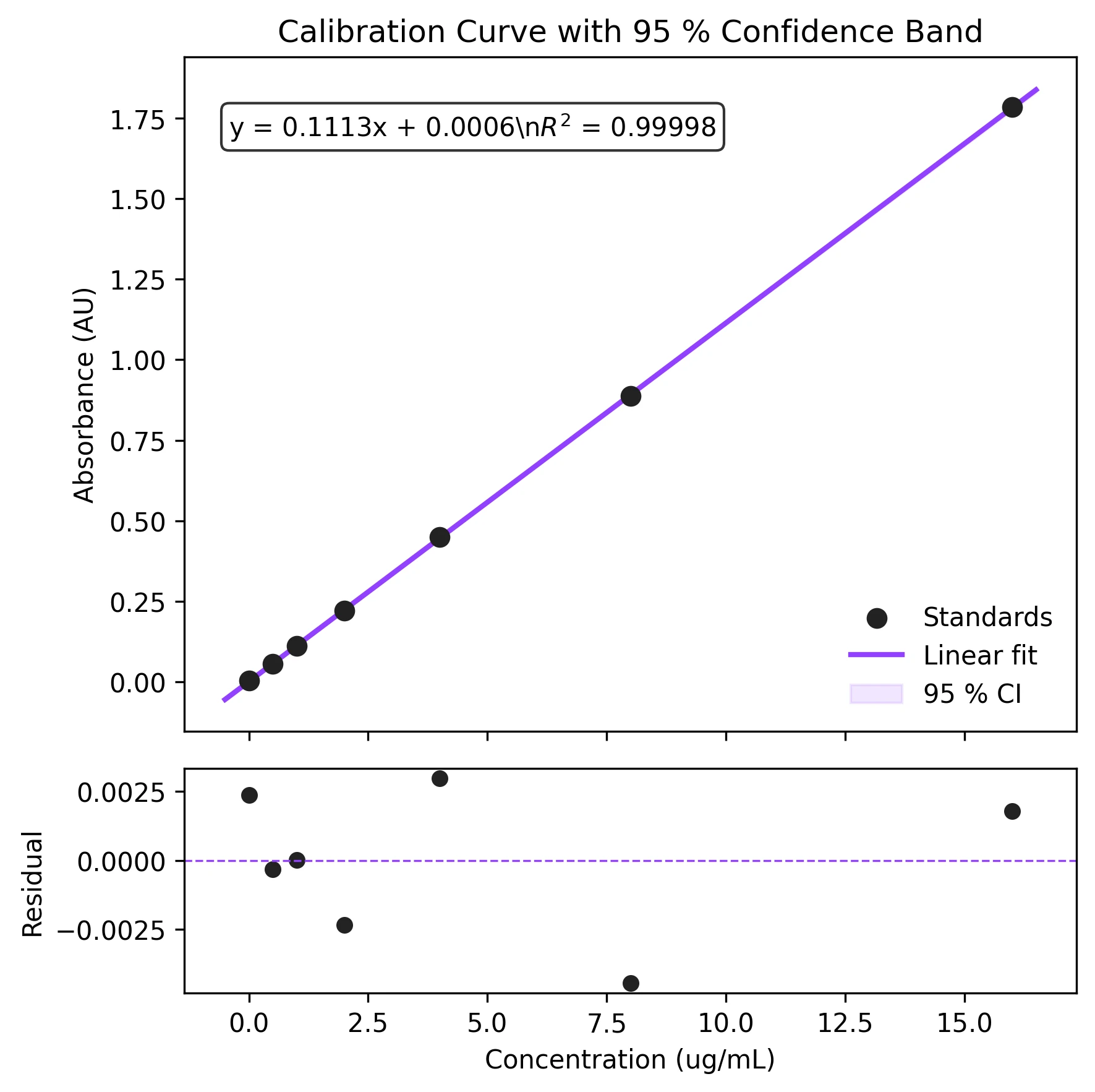
Build calibration curves and standard curves with linear regression. Includes confidence interval bands, R-squared annotation, and residual diagnostics.

Linear regression is the foundation of quantitative analytical chemistry. Every time you build a calibration curve for an ELISA plate reader, construct a standard curve for ICP-OES concentrations, or validate a spectrophotometric method against Beer-Lambert law, you are fitting a straight line and extracting a slope and intercept. The challenge is not the fit itself - it is presenting the result with proper confidence intervals, checking the residuals for model violations, and knowing when a weighted or log-linear model is more appropriate. This page provides the complete Python workflow from raw standards to a publication-ready calibration figure.

Key points

Build calibration curves and standard curves with linear regression. Includes confidence interval bands, R-squared annotation, and residual diagnostics.
Linear regression is the foundation of quantitative analytical chemistry.
Every time you build a calibration curve for an ELISA plate reader, construct a standard curve for ICP-OES concentrations, or validate a spectrophotometric method against Beer-Lambert law, you are fitting a straight line and extracting a slope and intercept.
The challenge is not the fit itself - it is presenting the result with proper confidence intervals, checking the residuals for model violations, and knowing when a weighted or log-linear model is more appropriate.

scipynumpymatplotlibstatsmodels

Example Visualization

Open full screen

Review the example first, then use the live editor below to run and customize the full workflow.

Mathematical Foundation

Linear regression is the foundation of quantitative analytical chemistry.

Equation

y = m * x + b

Parameter breakdown

mSlope (sensitivity of the method, e.g., absorbance per concentration unit)

bIntercept (blank signal or systematic offset)

R²Coefficient of determination; fraction of variance in y explained by the linear model

CI(y)Prediction confidence interval on ŷ: ŷ ± t(α/2, n−2) · sₑ · √[1/n + (x−x̄)²/SSₓ]

When to use this technique

Use ordinary least-squares (OLS) linear regression when the relationship between x and y is approximately linear, the residuals are normally distributed with constant variance, and the x-values are measured without significant error. If variance increases with concentration, use weighted least-squares instead.

Apply This Technique Now

Run this analysis workflow with AI in seconds. Use the prepared technique prompt or bring your own dataset.

Try Technique Prompt Use Your Own Data

View example prompt

Example AI Prompt

"Perform linear regression on my calibration data, show the fit line with 95% confidence bands, residuals subplot, and annotate R-squared and equation on the figure"

How to apply this technique in 30 seconds

Upload Data

Upload your CSV or Excel file in Analyze and keep your column names as-is.

Generate

Run the example prompt and let AI generate this technique automatically.

Refine and Export

Adjust code or prompt, then export publication-ready figures.

Implementation Code

The core data processing logic. Copy this block and replace the sample data with your measurements.

import numpy as np
from scipy import stats

# --- Calibration standards ---
concentrations = np.array([0.0, 0.5, 1.0, 2.0, 4.0, 8.0, 16.0])  # ug/mL
absorbances    = np.array([0.003, 0.056, 0.112, 0.221, 0.449, 0.887, 1.784])

# --- Linear regression ---
result = stats.linregress(concentrations, absorbances)
slope, intercept, r_value, p_value, std_err = result
r_squared = r_value ** 2

print(f"Slope     : {slope:.5f} +/- {std_err:.5f}")
print(f"Intercept : {intercept:.5f}")
print(f"R-squared : {r_squared:.6f}")
print(f"p-value   : {p_value:.2e}")

# --- Predict unknown concentration from measured absorbance ---
unknown_abs = 0.350
unknown_conc = (unknown_abs - intercept) / slope
print(f"\nUnknown at A={unknown_abs}: {unknown_conc:.3f} ug/mL")

Visualize This Implementation in Analyze

Visualization Code

Complete matplotlib code for a publication-ready figure. Copy, paste into your notebook, and adjust labels to match your data.

import numpy as np
import matplotlib.pyplot as plt
from scipy import stats

# --- Data ---
conc = np.array([0.0, 0.5, 1.0, 2.0, 4.0, 8.0, 16.0])
abso = np.array([0.003, 0.056, 0.112, 0.221, 0.449, 0.887, 1.784])

res = stats.linregress(conc, abso)
slope, intercept, r_value = res.slope, res.intercept, res.rvalue
r_sq = r_value ** 2

# --- Confidence band ---
n = len(conc)
x_fit = np.linspace(conc.min() - 0.5, conc.max() + 0.5, 200)
y_fit = slope * x_fit + intercept
y_pred = slope * conc + intercept
residuals = abso - y_pred
s_e = np.sqrt(np.sum(residuals ** 2) / (n - 2))
ss_x = np.sum((conc - conc.mean()) ** 2)
t_val = stats.t.ppf(0.975, n - 2)
ci = t_val * s_e * np.sqrt(1.0 / n + (x_fit - conc.mean()) ** 2 / ss_x)

# --- Figure ---
fig, (ax1, ax2) = plt.subplots(2, 1, figsize=(6, 6),
                                gridspec_kw={'height_ratios': [3, 1]},
                                sharex=True)
ax1.scatter(conc, abso, s=50, color='#222222', zorder=5, label='Standards')
ax1.plot(x_fit, y_fit, color='#9240ff', lw=2, label='Linear fit')
ax1.fill_between(x_fit, y_fit - ci, y_fit + ci, color='#9240ff', alpha=0.12,
                 label='95 % CI')
eq_text = f'y = {slope:.4f}x + {intercept:.4f}\n$R^2$ = {r_sq:.5f}'
ax1.text(0.05, 0.92, eq_text, transform=ax1.transAxes, fontsize=10,
         verticalalignment='top', bbox=dict(boxstyle='round', fc='white', alpha=0.8))
ax1.set_ylabel('Absorbance (AU)')
ax1.legend(frameon=False, loc='lower right')
ax1.set_title('Calibration Curve with 95 % Confidence Band', fontsize=12)

ax2.scatter(conc, residuals, s=30, color='#222222')
ax2.axhline(0, color='#9240ff', lw=0.8, ls='--')
ax2.set_xlabel('Concentration (ug/mL)')
ax2.set_ylabel('Residual')
plt.tight_layout()
plt.savefig('calibration_curve.png', dpi=300, bbox_inches='tight')
plt.show()

Visualize This Code in Analyze

Log-Linear Regression for Biological Data

Many biological assays (qPCR standard curves, growth curves in log phase) follow a log-linear relationship: log(y) = m * x + b, or y = m * log(x) + b. Transforming one axis before fitting linearises the data and lets you extract meaningful parameters such as PCR efficiency or doubling time.

import numpy as np
import matplotlib.pyplot as plt
from scipy import stats

# --- qPCR standard curve: Ct vs log10(copy number) ---
log_copies = np.array([1, 2, 3, 4, 5, 6, 7])        # log10 scale
ct_values  = np.array([32.1, 28.8, 25.4, 22.1, 18.7, 15.3, 11.9])

res = stats.linregress(log_copies, ct_values)
slope, intercept = res.slope, res.intercept
efficiency = (10 ** (-1 / slope) - 1) * 100

x_fit = np.linspace(0.5, 7.5, 200)
y_fit = slope * x_fit + intercept

# Residuals
residuals = ct_values - (slope * log_copies + intercept)

fig, (ax1, ax2) = plt.subplots(2, 1, figsize=(6, 5),
                                gridspec_kw={'height_ratios': [3, 1]},
                                sharex=True)
ax1.scatter(log_copies, ct_values, s=50, color='#222', zorder=5)
ax1.plot(x_fit, y_fit, color='#9240ff', lw=2)
ax1.set_ylabel('Ct value')
note = f'Slope = {slope:.2f}\nEfficiency = {efficiency:.1f} %\n$R^2$ = {res.rvalue**2:.5f}'
ax1.text(0.65, 0.92, note, transform=ax1.transAxes, fontsize=9,
         va='top', bbox=dict(boxstyle='round', fc='white', alpha=0.8))
ax1.set_title('qPCR Standard Curve (Log-Linear)', fontsize=12)

ax2.scatter(log_copies, residuals, s=30, color='#222')
ax2.axhline(0, color='#9240ff', lw=0.8, ls='--')
ax2.set_xlabel('log10(Copy Number)')
ax2.set_ylabel('Residual')
plt.tight_layout()
plt.savefig('log_linear_regression.png', dpi=300, bbox_inches='tight')
plt.show()

Visualize This Advanced Variant

Common Errors and How to Fix Them

Residuals fan out with increasing x (heteroscedasticity)

Why: Measurement variance grows with concentration, violating the constant-variance assumption of OLS.

Fix: Use weighted least-squares (WLS) with weights = 1/variance or 1/x^2, or transform the response (e.g., log transform) before fitting.

Residuals are not normally distributed (heavy tails or skewness)

Why: Outliers or a non-linear relationship can distort the residual distribution.

Fix: Check a Q-Q plot. Remove or investigate outliers. If the relationship is curved, consider a polynomial or weighted model.

One data point dramatically changes the slope (influential outlier)

Why: A leverage point at an extreme x-value with a large residual exerts disproportionate influence.

Fix: Compute Cook's distance for each point. If Cook's D > 4/n, investigate the point. Report results with and without it.

Extrapolating beyond the calibration range

Why: The linear relationship may not hold outside the measured concentration range.

Fix: Only interpolate within the range of your standards. Extend the calibration if higher or lower concentrations are needed.

Forcing the intercept through zero when it should not be

Why: Occasionally analysts assume b = 0 for calibration curves, but a non-zero blank is common.

Fix: Fit with a free intercept first. Only fix b = 0 if the intercept is not statistically different from zero (p > 0.05) and there is a physical reason.

Frequently Asked Questions

Apply Linear Regression in Python with Confidence Intervals to Your Data

Upload your dataset and Plotivy generates the Python code, runs the analysis, and produces a publication-ready figure.

Generate Code for This Technique

Python Libraries