Exponential Decay Fitting in Python
Technique overview
Fit single and double exponential decay models to extract rate constants, half-lives, and time constants from fluorescence, pharmacokinetics, or radioactive decay data.
Exponential decay is one of the most fundamental processes in quantitative science. Radioactive nuclei, excited fluorophores, drug plasma concentrations, and capacitor discharge all follow the same mathematical form: a quantity that decreases at a rate proportional to its current value. Extracting the decay time constant tau and the derived half-life from time-resolved measurements is therefore a universal task spanning nuclear physics, fluorescence lifetime imaging (FLIM), pharmacokinetics, and materials science. This page provides a complete Python workflow using scipy.optimize.curve_fit to fit single and double exponential models, extract tau and its uncertainty, compute the half-life with error propagation, and produce a publication-ready figure with a residuals panel.
Key points
- Fit single and double exponential decay models to extract rate constants, half-lives, and time constants from fluorescence, pharmacokinetics, or radioactive decay data.
- Exponential decay is one of the most fundamental processes in quantitative science.
- Radioactive nuclei, excited fluorophores, drug plasma concentrations, and capacitor discharge all follow the same mathematical form: a quantity that decreases at a rate proportional to its current value.
- Extracting the decay time constant tau and the derived half-life from time-resolved measurements is therefore a universal task spanning nuclear physics, fluorescence lifetime imaging (FLIM), pharmacokinetics, and materials science.
Example Visualization
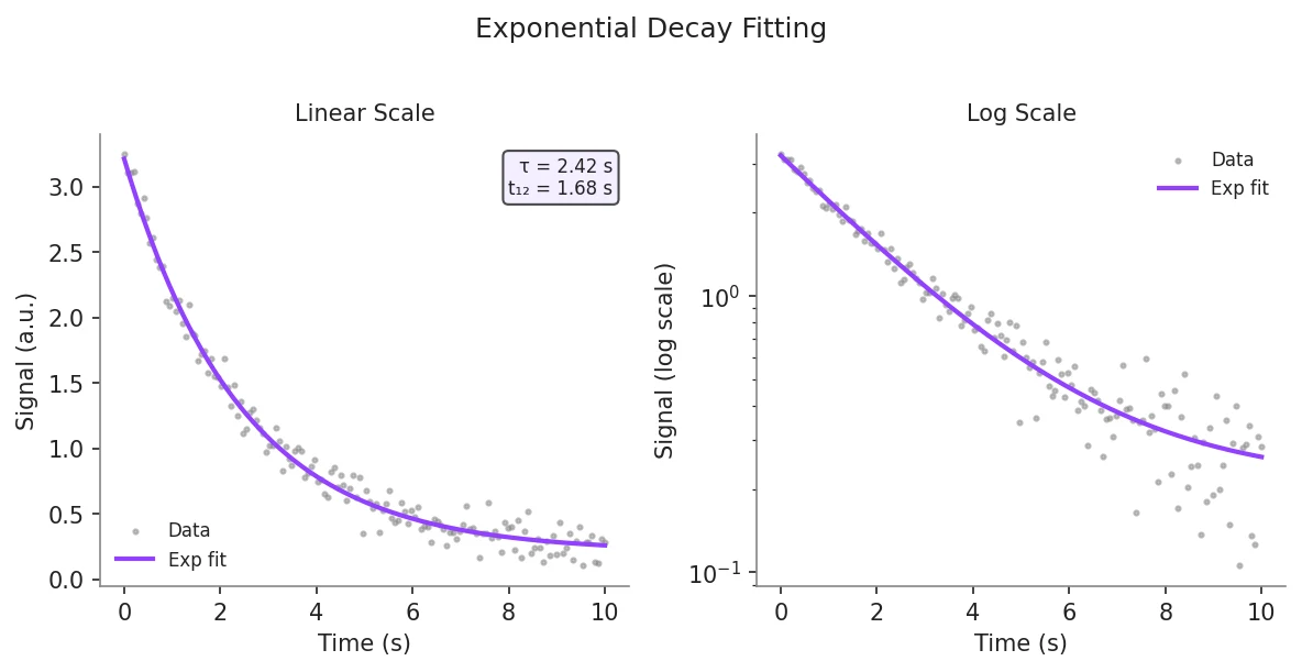
Review the example first, then use the live editor below to run and customize the full workflow.
Mathematical Foundation
Exponential decay is one of the most fundamental processes in quantitative science.
Equation
y(t) = A * exp(-t / tau) + CParameter breakdown
When to use this technique
Use a single exponential when only one decay process is present, indicated by a straight line on a semi-logarithmic plot of ln(y - C) vs t. If the semi-log plot is curved (concave upward), two processes with different rates are likely present, and a double exponential model (biexponential) should be considered. Avoid fitting exponentials to data with fewer than 20 points, as parameter covariance will be high.
Apply This Technique Now
Run this analysis workflow with AI in seconds. Use the prepared technique prompt or bring your own dataset.
View example prompt
"Fit an exponential decay to my time-series data, extract the decay time constant and half-life with 95% confidence intervals, and plot the data with fitted curve and residuals"
How to apply this technique in 30 seconds
Generate
Run the example prompt and let AI generate this technique automatically.
Refine and Export
Adjust code or prompt, then export publication-ready figures.
Implementation Code
The core data processing logic. Copy this block and replace the sample data with your measurements.
import numpy as np
from scipy.optimize import curve_fit

# --- Define single exponential decay model ---
def exp_decay(t, amplitude, tau, baseline):
    return amplitude * np.exp(-t / tau) + baseline

# --- Simulated fluorescence decay data ---
np.random.seed(42)
t_data = np.linspace(0, 50, 100)
y_true = exp_decay(t_data, amplitude=2.5, tau=10.0, baseline=0.1)
y_data = y_true + np.random.normal(0, 0.08, size=t_data.shape)
y_data = np.clip(y_data, 0, None)  # signal cannot be negative

# --- Initial guesses ---
# amplitude ~ max(y), tau ~ rough visual estimate, baseline ~ min(y)
p0 = [y_data.max() - y_data.min(), 8.0, y_data.min()]
bounds = ([0, 0.01, -np.inf], [np.inf, np.inf, np.inf])

# --- Fit ---
popt, pcov = curve_fit(exp_decay, t_data, y_data, p0=p0, bounds=bounds)
perr = np.sqrt(np.diag(pcov))

amp, tau_fit, baseline_fit = popt
amp_err, tau_err, baseline_err = perr
half_life = tau_fit * np.log(2)
half_life_err = tau_err * np.log(2)  # error propagation

print(f"Amplitude : {amp:.4f} +/- {amp_err:.4f}")
print(f"Tau       : {tau_fit:.4f} +/- {tau_err:.4f} s")
print(f"Half-life : {half_life:.4f} +/- {half_life_err:.4f} s")
print(f"Baseline : {baseline_fit:.4f} +/- {baseline_err:.4f}")Visualization Code
Complete matplotlib code for a publication-ready figure. Copy, paste into your notebook, and adjust labels to match your data.
import numpy as np
import matplotlib.pyplot as plt
from scipy.optimize import curve_fit

def exp_decay(t, amplitude, tau, baseline):
    return amplitude * np.exp(-t / tau) + baseline

# --- Data ---
np.random.seed(42)
t_data = np.linspace(0, 50, 100)
y_true = exp_decay(t_data, 2.5, 10.0, 0.1)
y_data = y_true + np.random.normal(0, 0.08, size=t_data.shape)
y_data = np.clip(y_data, 0, None)

p0 = [y_data.max() - y_data.min(), 8.0, y_data.min()]
bounds = ([0, 0.01, -np.inf], [np.inf, np.inf, np.inf])
popt, pcov = curve_fit(exp_decay, t_data, y_data, p0=p0, bounds=bounds)
perr = np.sqrt(np.diag(pcov))
y_fit = exp_decay(t_data, *popt)
residuals = y_data - y_fit
tau_fit, tau_err = popt[1], perr[1]
half_life = tau_fit * np.log(2)
half_life_err = tau_err * np.log(2)

# --- Figure ---
fig, axes = plt.subplots(2, 2, figsize=(10, 7),
                          gridspec_kw={'height_ratios': [3, 1],
                                       'width_ratios': [1, 1]})
for ax in axes.flat:
    ax.spines['top'].set_visible(False)
    ax.spines['right'].set_visible(False)

# Top-left: linear scale
ax1 = axes[0, 0]
ax1.scatter(t_data, y_data, s=8, color='#888888', alpha=0.6, label='Data')
ax1.plot(t_data, y_fit, color='#9240ff', linewidth=2, label='Exponential fit')
ax1.axvline(tau_fit, color='#9240ff', linestyle=':', linewidth=1, alpha=0.6)
ax1.axhline(y_fit[-1] + (y_fit[0] - y_fit[-1]) / np.e, color='gray',
            linestyle='--', linewidth=0.8, alpha=0.5)
ax1.set_ylabel('Signal (a.u.)', fontsize=11)
ax1.legend(frameon=False, fontsize=9)
ax1.set_title('Linear Scale', fontsize=11)
param_text = (f'tau = {tau_fit:.2f} +/- {tau_err:.2f} s\n'
              f't(1/2) = {half_life:.2f} +/- {half_life_err:.2f} s')
ax1.text(0.97, 0.95, param_text, transform=ax1.transAxes, fontsize=8,
         va='top', ha='right', color='white',
         bbox=dict(boxstyle='round', facecolor='#1a1a2e', alpha=0.6))

# Top-right: semi-log scale
ax2 = axes[0, 1]
y_above_baseline = y_data - popt[2]
valid = y_above_baseline > 0
ax2.semilogy(t_data[valid], y_above_baseline[valid], 'o', markersize=4,
             color='#888888', alpha=0.6, label='Data - baseline')
ax2.semilogy(t_data, exp_decay(t_data, popt[0], popt[1], 0),
             color='#9240ff', linewidth=2, label='Fit')
ax2.set_ylabel('Signal - baseline (log)', fontsize=11)
ax2.legend(frameon=False, fontsize=9)
ax2.set_title('Semi-log Scale', fontsize=11)

# Bottom row: residuals
for ax, res in zip(axes[1], [residuals, residuals]):
    ax.scatter(t_data, res, s=6, color='#888888', alpha=0.5)
    ax.axhline(0, color='#9240ff', linewidth=0.8, linestyle='--')
    ax.set_xlabel('Time (s)', fontsize=11)
    ax.set_ylabel('Residual', fontsize=10)

fig.suptitle('Exponential Decay Fit', fontsize=14, y=1.01)
plt.tight_layout()
plt.savefig('exponential_decay_fit.png', dpi=300, bbox_inches='tight')
plt.show()Double Exponential (Biexponential) Decay Fitting
Many fluorescence and pharmacokinetic datasets contain two distinct decay processes with different time constants. Fitting a biexponential model separates the fast and slow components and provides the fractional amplitude of each, giving mechanistic insight into the system. The amplitude-weighted mean lifetime is commonly reported for FLIM data.
import numpy as np
import matplotlib.pyplot as plt
from scipy.optimize import curve_fit

def biexp_decay(t, A1, tau1, A2, tau2, C):
    """Double exponential with baseline."""
    return A1 * np.exp(-t / tau1) + A2 * np.exp(-t / tau2) + C

# --- Synthetic biexponential data ---
np.random.seed(42)
t = np.linspace(0, 80, 160)
y_true = biexp_decay(t, A1=1.8, tau1=5.0, A2=0.8, tau2=25.0, C=0.05)
y = y_true + np.random.normal(0, 0.06, size=t.shape)
y = np.clip(y, 0, None)

# --- Initial guesses (fast + slow component) ---
p0 = [1.5, 4.0, 0.7, 20.0, 0.05]
bounds = ([0, 0.1, 0, 1.0, -np.inf], [np.inf, np.inf, np.inf, np.inf, np.inf])
popt, pcov = curve_fit(biexp_decay, t, y, p0=p0, bounds=bounds, maxfev=20000)
perr = np.sqrt(np.diag(pcov))

A1, tau1, A2, tau2 = popt[0], popt[1], popt[2], popt[3]
# Amplitude-weighted mean lifetime
tau_mean = (A1 * tau1 + A2 * tau2) / (A1 + A2)
frac1 = A1 / (A1 + A2)

print(f"Component 1: A={A1:.3f}, tau={tau1:.3f} s ({frac1*100:.1f}% fraction)")
print(f"Component 2: A={A2:.3f}, tau={tau2:.3f} s ({(1-frac1)*100:.1f}% fraction)")
print(f"Mean lifetime: {tau_mean:.3f} s")

fig, ax = plt.subplots(figsize=(7, 4))
ax.spines['top'].set_visible(False)
ax.spines['right'].set_visible(False)
ax.scatter(t, y, s=6, color='#888', alpha=0.5, label='Data')
ax.plot(t, biexp_decay(t, *popt), color='#9240ff', lw=2, label='Biexp fit')
ax.plot(t, A1 * np.exp(-t/tau1) + popt[4], '--', lw=1.2, label=f'Fast: tau={tau1:.1f}s')
ax.plot(t, A2 * np.exp(-t/tau2) + popt[4], '--', lw=1.2, label=f'Slow: tau={tau2:.1f}s')
ax.legend(frameon=False, fontsize=9)
ax.set_xlabel('Time (s)', fontsize=11)
ax.set_ylabel('Signal (a.u.)', fontsize=11)
ax.set_title('Biexponential Decay Decomposition', fontsize=13)
plt.tight_layout()
plt.savefig('biexponential_fit.png', dpi=300, bbox_inches='tight')
plt.show()Common Errors and How to Fix Them
Fitted tau is negative or unrealistically small
Why: Without a lower bound on tau, the optimizer can assign a negative time constant, which is physically meaningless. This often occurs when the initial guesses are far from the true values.
Fix: Always set bounds=([0, 0.01, -inf], [inf, inf, inf]) to enforce positive amplitude and tau. Estimate tau visually from the time at which the signal has dropped to ~37% of its range above baseline.
Optimizer converges to a flat line (tau extremely large)
Why: The data may not span a long enough time range to capture the full decay, leaving tau unconstrained. Alternatively, the baseline C is incorrectly estimated and the signal never appears to decay relative to it.
Fix: Ensure the data extends to at least 3-5 tau so the signal approaches the true baseline. Estimate C from the final few data points and use it as a fixed value or a tightly bounded parameter.
RuntimeWarning: covariance of the parameters could not be estimated
Why: The Jacobian is singular, which happens when two parameters trade off perfectly (e.g., A and tau in a biexponential with similar time constants) or when the noise is very high relative to the signal.
Fix: For biexponential fits, ensure the two time constants differ by at least a factor of 3. If pcov is inf, report only the point estimate and note that the uncertainty could not be estimated from the available data.
Frequently Asked Questions
Apply Exponential Decay Fitting in Python to Your Data
Upload your dataset and Plotivy generates the Python code, runs the analysis, and produces a publication-ready figure.
Generate Code for This TechniquePython Libraries
Quick Info
- Domain
- Curve Fitting
- Typical Audience
- Biophysicists, pharmacokineticists, and fluorescence spectroscopists extracting decay time constants from time-resolved experimental data