Kaplan-Meier Survival Analysis in Python
Technique overview
Estimate survival functions from censored time-to-event data with confidence intervals and log-rank tests for group comparison.
Survival analysis addresses a class of data that standard statistical methods cannot handle correctly: time-to-event outcomes where not all subjects have yet experienced the event by the end of the study. Patients who are still alive at last follow-up, participants who withdrew from a trial, or electronic components still functioning when the test ended all contribute partial information known as censored observations. Discarding these observations would bias the analysis toward shorter survival times. The Kaplan-Meier (product-limit) estimator is the standard non-parametric method for incorporating censored data, producing a step-function estimate of the survival probability S(t) over time. It is ubiquitous in clinical oncology, device reliability engineering, and epidemiology, and pairing it with the log-rank test allows rigorous group comparison. This page demonstrates the complete Python workflow using numpy and scipy - no third-party survival analysis packages required.
Key points
- Estimate survival functions from censored time-to-event data with confidence intervals and log-rank tests for group comparison.
- Survival analysis addresses a class of data that standard statistical methods cannot handle correctly: time-to-event outcomes where not all subjects have yet experienced the event by the end of the study.
- Patients who are still alive at last follow-up, participants who withdrew from a trial, or electronic components still functioning when the test ended all contribute partial information known as censored observations.
- Discarding these observations would bias the analysis toward shorter survival times.
Example Visualization
Review the example first, then use the live editor below to run and customize the full workflow.
Mathematical Foundation
Survival analysis addresses a class of data that standard statistical methods cannot handle correctly: time-to-event outcomes where not all subjects have yet experienced the event by the end of the study.
Equation
S(t) = product_{ti <= t} [ (ni - di) / ni ]Parameter breakdown
When to use this technique
Use Kaplan-Meier analysis whenever you have time-to-event data with censoring. It is appropriate for clinical endpoints (overall survival, progression-free survival), reliability endpoints (time to failure), and any study where subjects enter and exit the observation window at different times. For adjusted estimates that control for covariates, use the Cox proportional hazards model as an extension.
Apply This Technique Now
Run this analysis workflow with AI in seconds. Use the prepared technique prompt or bring your own dataset.
View example prompt
"Plot Kaplan-Meier survival curves for my censored time-to-event data, add 95% confidence intervals, perform a log-rank test for group comparison, and annotate the median survival time for each group"
How to apply this technique in 30 seconds
Generate
Run the example prompt and let AI generate this technique automatically.
Refine and Export
Adjust code or prompt, then export publication-ready figures.
Implementation Code
The core data processing logic. Copy this block and replace the sample data with your measurements.
import numpy as np
from scipy import stats as scipy_stats

def kaplan_meier(durations, event_observed):
    """Compute Kaplan-Meier survival estimate via the product-limit formula."""
    durations = np.asarray(durations, dtype=float)
    event_observed = np.asarray(event_observed, dtype=bool)
    order = np.argsort(durations)
    durations, event_observed = durations[order], event_observed[order]
    n = len(durations)
    times, survival = [0.0], [1.0]
    n_at_risk = n
    i = 0
    while i < n:
        t = durations[i]
        j = i
        while j < n and durations[j] == t:
            j += 1
        d = int(event_observed[i:j].sum())
        if d > 0:
            times.append(t)
            survival.append(survival[-1] * (1.0 - d / n_at_risk))
        n_at_risk -= (j - i)
        i = j
    return np.array(times), np.array(survival)

def km_median(times, survival):
    """First time at which S(t) <= 0.5 (median survival)."""
    idx = np.where(survival <= 0.5)[0]
    return times[idx[0]] if len(idx) > 0 else float('inf')

def log_rank_test(t1, e1, t2, e2):
    """Chi-squared log-rank test for two independent groups."""
    e1, e2 = np.asarray(e1, bool), np.asarray(e2, bool)
    event_times = np.unique(np.concatenate([t1[e1], t2[e2]]))
    O1, E1, V = 0.0, 0.0, 0.0
    for t in event_times:
        n1, n2 = int((t1 >= t).sum()), int((t2 >= t).sum())
        d1, d2 = int(((t1 == t) & e1).sum()), int(((t2 == t) & e2).sum())
        n, d = n1 + n2, d1 + d2
        if n > 1:
            E1 += n1 * d / n
            O1 += d1
            V += n1 * n2 * d * (n - d) / (n ** 2 * (n - 1))
    chi2 = (O1 - E1) ** 2 / (V + 1e-15)
    p_val = float(1 - scipy_stats.chi2.cdf(chi2, df=1))
    return chi2, p_val

# --- Two-group survival data ---
np.random.seed(42)
n_per_group = 50

durations_a = np.random.exponential(scale=18, size=n_per_group)
events_a    = np.random.binomial(1, 0.75, size=n_per_group)  # 75% observed events

durations_b = np.random.exponential(scale=10, size=n_per_group)
events_b    = np.random.binomial(1, 0.80, size=n_per_group)  # 80% observed events

t_a, s_a = kaplan_meier(durations_a, events_a)
t_b, s_b = kaplan_meier(durations_b, events_b)

print(f"Median survival - Group A: {km_median(t_a, s_a):.2f} months")
print(f"Median survival - Group B: {km_median(t_b, s_b):.2f} months")

chi2, p_value = log_rank_test(durations_a, events_a, durations_b, events_b)
print(f"\nLog-rank test:")
print(f"  Test statistic : {chi2:.4f}")
print(f"  p-value        : {p_value:.4f}")
sig = '***' if p_value < 0.001 else ('**' if p_value < 0.01 else ('*' if p_value < 0.05 else 'ns'))
print(f" Significance : {sig}")Visualization Code
Complete matplotlib code for a publication-ready figure. Copy, paste into your notebook, and adjust labels to match your data.
import numpy as np
import matplotlib.pyplot as plt
from scipy import stats as scipy_stats
def kaplan_meier(durations, event_observed):
durations = np.asarray(durations, dtype=float)
event_observed = np.asarray(event_observed, dtype=bool)
order = np.argsort(durations)
durations, event_observed = durations[order], event_observed[order]
n = len(durations)
times, survival = [0.0], [1.0]
n_at_risk = n
i = 0
while i < n:
t = durations[i]
j = i
while j < n and durations[j] == t:
j += 1
d = int(event_observed[i:j].sum())
if d > 0:
times.append(t)
survival.append(survival[-1] * (1.0 - d / n_at_risk))
n_at_risk -= (j - i)
i = j
return np.array(times), np.array(survival)
def km_median(times, survival):
idx = np.where(survival <= 0.5)[0]
return times[idx[0]] if len(idx) > 0 else float('inf')
def log_rank_p(t1, e1, t2, e2):
e1, e2 = np.asarray(e1, bool), np.asarray(e2, bool)
event_times = np.unique(np.concatenate([t1[e1], t2[e2]]))
O1, E1, V = 0.0, 0.0, 0.0
for t in event_times:
n1, n2 = int((t1 >= t).sum()), int((t2 >= t).sum())
d1, d2 = int(((t1 == t) & e1).sum()), int(((t2 == t) & e2).sum())
n, d = n1 + n2, d1 + d2
if n > 1:
E1 += n1 * d / n
O1 += d1
V += n1 * n2 * d * (n - d) / (n ** 2 * (n - 1))
chi2 = (O1 - E1) ** 2 / (V + 1e-15)
return float(1 - scipy_stats.chi2.cdf(chi2, df=1))
# --- Data ---
np.random.seed(42)
n = 50
durations_a = np.random.exponential(scale=18, size=n)
events_a = np.random.binomial(1, 0.75, size=n)
durations_b = np.random.exponential(scale=10, size=n)
events_b = np.random.binomial(1, 0.80, size=n)
t_a, s_a = kaplan_meier(durations_a, events_a)
t_b, s_b = kaplan_meier(durations_b, events_b)
p_val = log_rank_p(durations_a, events_a, durations_b, events_b)
sig = '***' if p_val < 0.001 else ('**' if p_val < 0.01 else ('*' if p_val < 0.05 else 'ns'))
# --- Figure ---
fig, ax = plt.subplots(figsize=(8, 5))
ax.spines['top'].set_visible(False)
ax.spines['right'].set_visible(False)
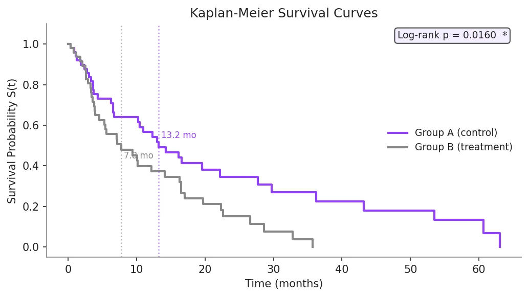
ax.step(t_a, s_a, where='post', color='#9240ff', linewidth=2, label='Group A (control)')
ax.step(t_b, s_b, where='post', color='#888888', linewidth=2, label='Group B (treatment)')
for t_km, s_km, color, y_pos in [(t_a, s_a, '#9240ff', 0.55), (t_b, s_b, '#888888', 0.45)]:
med = km_median(t_km, s_km)
if not np.isinf(med):
ax.axvline(med, color=color, linestyle=':', linewidth=1.2, alpha=0.7)
ax.text(med + 0.5, y_pos, f'Median = {med:.1f} mo',
color=color, fontsize=8.5, va='center')
ax.text(0.97, 0.97,
f'Log-rank test\np = {p_val:.4f} {sig}',
transform=ax.transAxes, ha='right', va='top',
fontsize=9, color='white',
bbox=dict(boxstyle='round', facecolor='#1a1a2e', alpha=0.7))
ax.set_xlabel('Time (months)', fontsize=12)
ax.set_ylabel('Survival Probability S(t)', fontsize=12)
ax.set_ylim(-0.05, 1.05)
ax.set_title('Kaplan-Meier Survival Curves', fontsize=14)
ax.legend(frameon=False, fontsize=10, loc='upper right',
bbox_to_anchor=(0.97, 0.80))
plt.tight_layout()
plt.savefig('kaplan_meier_survival.png', dpi=300, bbox_inches='tight')
plt.show()Stratified Kaplan-Meier with Three or More Groups
Clinical studies frequently stratify patients by multiple factors such as disease stage, treatment dose, or biomarker level. Plotting Kaplan-Meier curves for three or more groups simultaneously and using a multivariate log-rank test (or pairwise tests with Bonferroni correction) extends the two-group comparison to more complex study designs.
import numpy as np
import matplotlib.pyplot as plt
from scipy import stats as scipy_stats

def kaplan_meier(durations, event_observed):
    durations = np.asarray(durations, dtype=float)
    event_observed = np.asarray(event_observed, dtype=bool)
    order = np.argsort(durations)
    durations, event_observed = durations[order], event_observed[order]
    n = len(durations)
    times, survival = [0.0], [1.0]
    n_at_risk = n
    i = 0
    while i < n:
        t = durations[i]
        j = i
        while j < n and durations[j] == t:
            j += 1
        d = int(event_observed[i:j].sum())
        if d > 0:
            times.append(t)
            survival.append(survival[-1] * (1.0 - d / n_at_risk))
        n_at_risk -= (j - i)
        i = j
    return np.array(times), np.array(survival)

def multivariate_log_rank_p(all_dur, all_grp, all_ev):
    """Chi-squared log-rank test for K groups (K-1 degrees of freedom)."""
    all_dur = np.asarray(all_dur, float)
    all_ev  = np.asarray(all_ev, bool)
    unique_g = sorted(set(all_grp))
    K = len(unique_g)
    event_times = np.unique(all_dur[all_ev])
    O = np.zeros(K); E = np.zeros(K); V = np.zeros((K, K))
    for t in event_times:
        mask_r = all_dur >= t
        mask_e = (all_dur == t) & all_ev
        n_all = mask_r.sum(); d_all = mask_e.sum()
        if n_all < 2:
            continue
        n_k = np.array([mask_r[np.array(all_grp) == g].sum() for g in unique_g], float)
        d_k = np.array([mask_e[np.array(all_grp) == g].sum() for g in unique_g], float)
        O += d_k; E += n_k * d_all / n_all
        for i in range(K):
            V[i, i] += (n_k[i] * (n_all - n_k[i]) * d_all *
                        (n_all - d_all) / (n_all ** 2 * max(n_all - 1, 1)))
    diffs = (O - E)[:-1]
    Vs = V[:-1, :-1]
    try:
        chi2 = float(diffs @ np.linalg.inv(Vs) @ diffs)
    except np.linalg.LinAlgError:
        chi2 = 0.0
    return float(1 - scipy_stats.chi2.cdf(chi2, df=K - 1))

# --- Three-group survival data ---
np.random.seed(42)
n = 40
groups = {
    'Stage I (early)':    (np.random.exponential(24, n), np.random.binomial(1, 0.65, n)),
    'Stage II (mid)':     (np.random.exponential(14, n), np.random.binomial(1, 0.75, n)),
    'Stage III (late)':   (np.random.exponential(7,  n), np.random.binomial(1, 0.85, n)),
}
colors = ['#9240ff', '#888888', '#e8a020']

fig, ax = plt.subplots(figsize=(8, 5))
ax.spines['top'].set_visible(False)
ax.spines['right'].set_visible(False)

all_dur, all_ev, all_grp = [], [], []
for (label, (dur, ev)), color in zip(groups.items(), colors):
    t_km, s_km = kaplan_meier(dur, ev)
    ax.step(t_km, s_km, where='post', color=color, linewidth=2, label=label)
    all_dur.extend(dur.tolist())
    all_ev.extend(ev.tolist())
    all_grp.extend([label] * n)

p_val = multivariate_log_rank_p(np.array(all_dur), all_grp, np.array(all_ev))
sig = '***' if p_val < 0.001 else ('**' if p_val < 0.01 else ('*' if p_val < 0.05 else 'ns'))

ax.text(0.97, 0.97,
        f'Log-rank test (3 groups)\np = {p_val:.4f}  {sig}',
        transform=ax.transAxes, ha='right', va='top', fontsize=9, color='white',
        bbox=dict(boxstyle='round', facecolor='#1a1a2e', alpha=0.7))
ax.set_xlabel('Time (months)', fontsize=12)
ax.set_ylabel('Survival Probability S(t)', fontsize=12)
ax.set_ylim(-0.05, 1.05)
ax.set_title('Stratified Kaplan-Meier Survival Curves', fontsize=14)
ax.legend(frameon=False, fontsize=9, loc='upper right')
plt.tight_layout()
plt.savefig('kaplan_meier_stratified.png', dpi=300, bbox_inches='tight')
plt.show()Common Errors and How to Fix Them
median_survival_time returns inf
Why: The survival curve never crosses 0.5 within the observed time range. Fewer than 50% of subjects have experienced the event, so the median is not estimable from the available data.
Fix: Report the event as 'median not reached' or extend follow-up. You can still report survival probability at a specific landmark time by evaluating the step function: find the last time in the times array that is <= your landmark and read the corresponding survival value.
Log-rank test is significant but KM curves visually overlap
Why: The log-rank test is sensitive to differences at any time point, including at early or late time points where the curves may diverge temporarily. It weights all event times equally.
Fix: Check where in the follow-up the curves diverge by examining the timeline. If the difference occurs only at early times and then converges, the proportional hazards assumption may be violated - consider reporting restricted mean survival time (RMST) instead.
Frequently Asked Questions
Apply Kaplan-Meier Survival Analysis in Python to Your Data
Upload your dataset and Plotivy generates the Python code, runs the analysis, and produces a publication-ready figure.
Generate Code for This TechniquePython Libraries
Quick Info
- Domain
- Clinical
- Typical Audience
- Clinical researchers, epidemiologists, and biostatisticians analyzing time-to-event outcomes such as patient survival, device failure, or disease recurrence