Lorentzian Curve Fitting in Python
Technique overview
Fit Lorentzian (Cauchy) profiles to spectroscopy data with heavier tails than Gaussian peaks, common in NMR and Raman broadening.
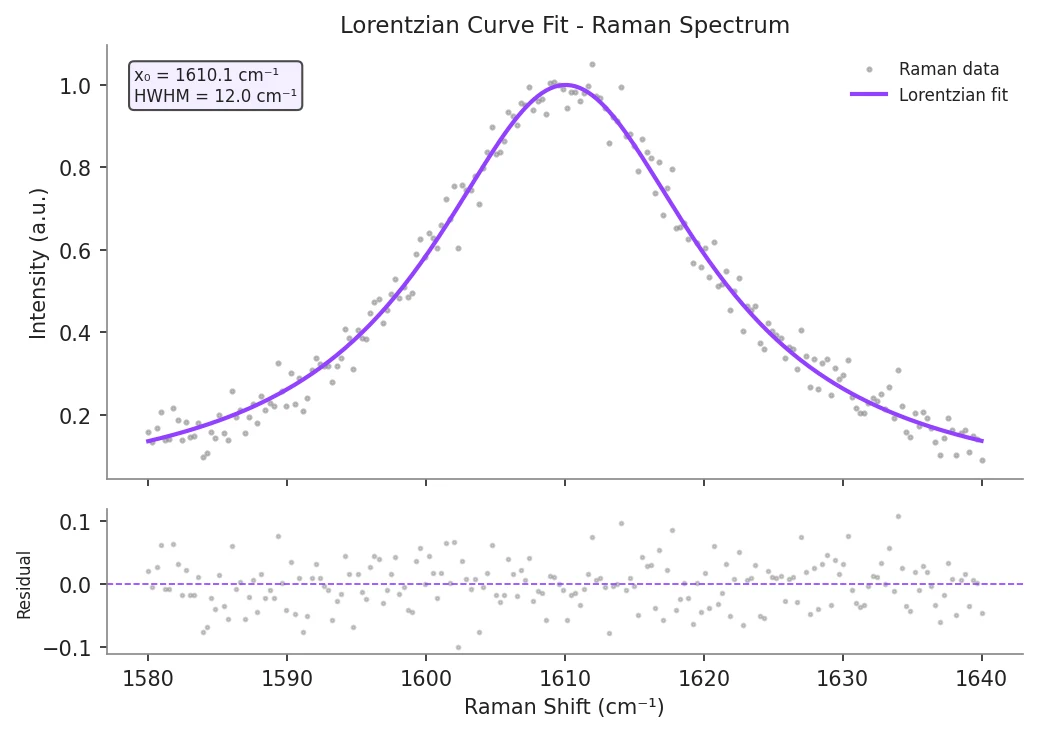
In spectroscopy, not all peaks are bell-shaped. When the broadening mechanism is homogeneous - caused by a finite excited-state lifetime, pressure collisions, or spin-spin relaxation in NMR - the resulting lineshape follows a Lorentzian (Cauchy) distribution rather than a Gaussian. Lorentzian peaks are taller and sharper at the center but fall off much more slowly in the wings, which means a Gaussian fit will systematically underestimate the intensity in the tails. This distinction matters in Raman spectroscopy, where phonon lifetime determines peak width, in NMR linewidth analysis, and in electron paramagnetic resonance. This page demonstrates how to fit a Lorentzian model in Python using scipy.optimize.curve_fit, extract the half-width at half-maximum (HWHM) with propagated uncertainties, and produce a publication-ready overlay with residuals.
Key points
- Fit Lorentzian (Cauchy) profiles to spectroscopy data with heavier tails than Gaussian peaks, common in NMR and Raman broadening.
- In spectroscopy, not all peaks are bell-shaped.
- When the broadening mechanism is homogeneous - caused by a finite excited-state lifetime, pressure collisions, or spin-spin relaxation in NMR - the resulting lineshape follows a Lorentzian (Cauchy) distribution rather than a Gaussian.
- Lorentzian peaks are taller and sharper at the center but fall off much more slowly in the wings, which means a Gaussian fit will systematically underestimate the intensity in the tails.
Example Visualization
Review the example first, then use the live editor below to run and customize the full workflow.
Mathematical Foundation
In spectroscopy, not all peaks are bell-shaped.
Equation
f(x) = A * gamma^2 / ((x - x0)^2 + gamma^2)Parameter breakdown
When to use this technique
Use a Lorentzian when your spectral peak arises from a homogeneous broadening mechanism such as natural linewidth, pressure broadening, or T2 relaxation in NMR. If both homogeneous and inhomogeneous broadening are present, consider a Voigt profile (convolution of Lorentzian and Gaussian). Compare the tail behavior of residuals from a Gaussian fit: systematic positive residuals in the wings indicate a Lorentzian is more appropriate.
Apply This Technique Now
Run this analysis workflow with AI in seconds. Use the prepared technique prompt or bring your own dataset.
View example prompt
"Fit a Lorentzian profile to my NMR or Raman spectroscopy data, extract peak position, amplitude, and HWHM with uncertainties, and overlay the fit on raw data with residuals"
How to apply this technique in 30 seconds
Generate
Run the example prompt and let AI generate this technique automatically.
Refine and Export
Adjust code or prompt, then export publication-ready figures.
Implementation Code
The core data processing logic. Copy this block and replace the sample data with your measurements.
import numpy as np
from scipy.optimize import curve_fit

# --- Define the Lorentzian model ---
def lorentzian(x, amplitude, center, gamma):
    """Lorentzian (Cauchy) profile."""
    return amplitude * gamma**2 / ((x - center)**2 + gamma**2)

# --- Simulated Raman spectroscopy data ---
np.random.seed(42)
x_data = np.linspace(1200, 1400, 201)
y_true = lorentzian(x_data, amplitude=0.9, center=1310.0, gamma=8.0)
y_data = y_true + np.random.normal(0, 0.025, size=x_data.shape)

# --- Initial parameter guesses ---
# amplitude ~ max of data, center ~ position of max, gamma ~ rough half-width
p0 = [y_data.max(), x_data[np.argmax(y_data)], 5.0]

# --- Fit with positive constraints ---
bounds = ([0, x_data.min(), 0.1], [np.inf, x_data.max(), np.inf])
popt, pcov = curve_fit(lorentzian, x_data, y_data, p0=p0, bounds=bounds)
perr = np.sqrt(np.diag(pcov))

print(f"Amplitude : {popt[0]:.4f} +/- {perr[0]:.4f}")
print(f"Center    : {popt[1]:.4f} +/- {perr[1]:.4f} cm-1")
print(f"HWHM      : {popt[2]:.4f} +/- {perr[2]:.4f} cm-1")
print(f"FWHM      : {2 * popt[2]:.4f} +/- {2 * perr[2]:.4f} cm-1")

# --- Residuals ---
y_fit = lorentzian(x_data, *popt)
residuals = y_data - y_fit
ss_res = np.sum(residuals**2)
ss_tot = np.sum((y_data - y_data.mean())**2)
print(f"R-squared : {1 - ss_res / ss_tot:.6f}")Visualization Code
Complete matplotlib code for a publication-ready figure. Copy, paste into your notebook, and adjust labels to match your data.
import numpy as np
import matplotlib.pyplot as plt
from scipy.optimize import curve_fit

def lorentzian(x, amplitude, center, gamma):
    return amplitude * gamma**2 / ((x - center)**2 + gamma**2)

# --- Data ---
np.random.seed(42)
x_data = np.linspace(1200, 1400, 201)
y_true = lorentzian(x_data, 0.9, 1310.0, 8.0)
y_data = y_true + np.random.normal(0, 0.025, size=x_data.shape)

bounds = ([0, x_data.min(), 0.1], [np.inf, x_data.max(), np.inf])
popt, pcov = curve_fit(lorentzian, x_data, y_data,
                       p0=[y_data.max(), x_data[np.argmax(y_data)], 5.0],
                       bounds=bounds)
perr = np.sqrt(np.diag(pcov))
y_fit = lorentzian(x_data, *popt)
residuals = y_data - y_fit

# --- 95% confidence band via bootstrap ---
n_boot = 500
y_boot = np.zeros((n_boot, len(x_data)))
for i in range(n_boot):
    p_s = np.random.multivariate_normal(popt, pcov)
    p_s[0] = max(p_s[0], 0)
    p_s[2] = max(p_s[2], 0.01)
    y_boot[i] = lorentzian(x_data, *p_s)
ci_low = np.percentile(y_boot, 2.5, axis=0)
ci_high = np.percentile(y_boot, 97.5, axis=0)

# --- Figure ---
fig, (ax1, ax2) = plt.subplots(2, 1, figsize=(7, 6),
                                gridspec_kw={'height_ratios': [3, 1]},
                                sharex=True)
for ax in (ax1, ax2):
    ax.spines['top'].set_visible(False)
    ax.spines['right'].set_visible(False)

ax1.scatter(x_data, y_data, s=8, color='#888888', alpha=0.6, label='Data')
ax1.plot(x_data, y_fit, color='#9240ff', linewidth=2, label='Lorentzian fit')
ax1.fill_between(x_data, ci_low, ci_high, color='#9240ff', alpha=0.15,
                 label='95% CI')
ax1.axvline(popt[1], color='#9240ff', linestyle=':', linewidth=1, alpha=0.7)
ax1.set_ylabel('Raman Intensity (a.u.)', fontsize=11)
ax1.legend(frameon=False, fontsize=9)
param_text = (f'Center = {popt[1]:.1f} +/- {perr[1]:.1f} cm$^{{-1}}$\n'
              f'HWHM = {popt[2]:.1f} +/- {perr[2]:.1f} cm$^{{-1}}$\n'
              f'FWHM = {2*popt[2]:.1f} cm$^{{-1}}$')
ax1.text(0.97, 0.95, param_text, transform=ax1.transAxes, fontsize=8,
         va='top', ha='right', color='white',
         bbox=dict(boxstyle='round', facecolor='#1a1a2e', alpha=0.6))
ax1.set_title('Lorentzian Curve Fit - Raman Spectrum', fontsize=13)

ax2.scatter(x_data, residuals, s=6, color='#888888', alpha=0.5)
ax2.axhline(0, color='#9240ff', linewidth=0.8, linestyle='--')
ax2.set_xlabel('Raman Shift (cm$^{-1}$)', fontsize=11)
ax2.set_ylabel('Residual', fontsize=10)

plt.tight_layout()
plt.savefig('lorentzian_fit.png', dpi=300, bbox_inches='tight')
plt.show()Multi-Peak Lorentzian Fitting
Raman and NMR spectra frequently contain two or more overlapping Lorentzian peaks. Fit a sum of Lorentzians simultaneously by parameterizing each peak with its own amplitude, center, and HWHM. Supplying tight initial guesses and parameter bounds for each component is essential to prevent the optimizer from merging degenerate components.
import numpy as np
import matplotlib.pyplot as plt
from scipy.optimize import curve_fit

def multi_lorentzian(x, *params):
    """Sum of N Lorentzians. params = [A1, x01, g1, A2, x02, g2, ...]"""
    y = np.zeros_like(x, dtype=float)
    for i in range(0, len(params), 3):
        A, x0, g = params[i], params[i+1], params[i+2]
        y += A * g**2 / ((x - x0)**2 + g**2)
    return y

# --- Synthetic two-peak Raman data ---
np.random.seed(7)
x = np.linspace(1250, 1450, 300)
y_true = (0.7 * 10**2 / ((x - 1300)**2 + 10**2) +
          1.0 * 12**2 / ((x - 1360)**2 + 12**2))
y = y_true + np.random.normal(0, 0.02, size=x.shape)

# --- Initial guesses: [A1, x01, g1, A2, x02, g2] ---
p0 = [0.6, 1300, 8, 0.9, 1360, 10]
lb = [0, 1250, 0.5, 0, 1300, 0.5]
ub = [2,  1330, 30,  2, 1420, 30]

popt, pcov = curve_fit(multi_lorentzian, x, y, p0=p0,
                       bounds=(lb, ub), maxfev=20000)
perr = np.sqrt(np.diag(pcov))

fig, ax = plt.subplots(figsize=(7, 4))
ax.spines['top'].set_visible(False)
ax.spines['right'].set_visible(False)
ax.scatter(x, y, s=6, color='#888', alpha=0.5, label='Data')
ax.plot(x, multi_lorentzian(x, *popt), color='#9240ff', lw=2, label='Sum fit')
for i in range(0, len(popt), 3):
    yi = popt[i] * popt[i+2]**2 / ((x - popt[i+1])**2 + popt[i+2]**2)
    ax.plot(x, yi, '--', lw=1.2, label=f'Peak {i//3 + 1}')
ax.legend(frameon=False, fontsize=9)
ax.set_xlabel('Raman Shift (cm$^{-1}$)', fontsize=11)
ax.set_ylabel('Intensity (a.u.)', fontsize=11)
ax.set_title('Multi-Peak Lorentzian Decomposition', fontsize=13)
plt.tight_layout()
plt.savefig('multi_lorentzian_fit.png', dpi=300, bbox_inches='tight')
plt.show()Common Errors and How to Fix Them
RuntimeError: Optimal parameters not found (maxfev exceeded)
Why: The initial guess for gamma (HWHM) is far from the true value, or the amplitude guess has the wrong order of magnitude, causing the optimizer to wander without converging.
Fix: Estimate gamma visually as half the observed peak width at half the peak height. Set bounds=([0, xmin, 0.1], [inf, xmax, inf]) to keep parameters physically meaningful and increase maxfev to 10000.
Fitted HWHM is unrealistically large (gamma >> peak width)
Why: Without an upper bound on gamma, the Lorentzian can approximate a flat baseline by making the peak extremely broad, which is a valid but physically meaningless solution.
Fix: Add an upper bound on gamma: bounds=([0, -inf, 0], [inf, inf, max_expected_width]). Subtract or model the baseline separately before fitting.
Fit looks correct visually but pcov diagonal contains inf
Why: The covariance matrix is ill-conditioned, usually because two parameters are highly correlated or the data do not span enough of the peak to constrain all three parameters independently.
Fix: Ensure the data range covers at least 5 * gamma on each side of the center. If the wings are not measured, fix gamma manually rather than fitting it.
Frequently Asked Questions
Apply Lorentzian Curve Fitting in Python to Your Data
Upload your dataset and Plotivy generates the Python code, runs the analysis, and produces a publication-ready figure.
Generate Code for This TechniquePython Libraries
Quick Info
- Domain
- Curve Fitting
- Typical Audience
- Spectroscopists, NMR chemists, and Raman analysts fitting peaks with homogeneous broadening or heavy tails that a Gaussian underestimates