Signal ProcessingLive Code Editor

110 researchers ran this analysis this month

Savitzky-Golay Smoothing in Python for Spectroscopy Data

Technique overview

Smooth spectroscopy and chromatography data while preserving peak shapes. Includes parameter selection guide for window length and polynomial order.

Noise is unavoidable in experimental science - a Raman spectrometer has shot noise, an FTIR instrument has detector noise, and an HPLC signal has electronic baseline drift. Savitzky-Golay filtering is the standard first-pass smoothing method because it preserves peak shapes, heights, and positions far better than a moving average. Instead of averaging neighbouring points equally, it fits a local polynomial to each window and uses the polynomial value at the center point, effectively acting as a low-pass filter that respects the underlying signal curvature. This page shows you how to choose the window length and polynomial order, visualize the effect of different parameters, and calculate smoothed derivatives for peak detection.

Key points

Smooth spectroscopy and chromatography data while preserving peak shapes. Includes parameter selection guide for window length and polynomial order.
Noise is unavoidable in experimental science - a Raman spectrometer has shot noise, an FTIR instrument has detector noise, and an HPLC signal has electronic baseline drift.
Savitzky-Golay filtering is the standard first-pass smoothing method because it preserves peak shapes, heights, and positions far better than a moving average.
Instead of averaging neighbouring points equally, it fits a local polynomial to each window and uses the polynomial value at the center point, effectively acting as a low-pass filter that respects the underlying signal curvature.

scipynumpymatplotlib

Example Visualization

Open full screen

Review the example first, then use the live editor below to run and customize the full workflow.

Mathematical Foundation

Noise is unavoidable in experimental science - a Raman spectrometer has shot noise, an FTIR instrument has detector noise, and an HPLC signal has electronic baseline drift.

Equation

y_smoothed[i] = sum_{j=-m}^{m} c_j * y[i+j]

Parameter breakdown

y_smoothed[i]Smoothed signal value at index i computed by the weighted local sum.

c_jConvolution weight for offset j inside the moving window; weights come from the local polynomial fit.

j = -m ... +mWindow offset index around i. The half-window size m is (window_length - 1) / 2.

window_length and polyordersavgol_filter hyperparameters used to derive c_j. window_length must be odd and polyorder < window_length.

When to use this technique

Use this when your raw signal is noisy but peak height, width, and position must stay physically meaningful. The implementation below uses window_length=15 and polyorder=3, which is a practical starting point for spectroscopy traces with moderate noise.

Apply This Technique Now

Run this analysis workflow with AI in seconds. Use the prepared technique prompt or bring your own dataset.

Try Technique Prompt Use Your Own Data

View example prompt

Example AI Prompt

"Smooth my spectroscopy data using Savitzky-Golay filter, show raw vs smoothed overlay, and compare different window sizes to find the best setting"

How to apply this technique in 30 seconds

Upload Data

Upload your CSV or Excel file in Analyze and keep your column names as-is.

Generate

Run the example prompt and let AI generate this technique automatically.

Refine and Export

Adjust code or prompt, then export publication-ready figures.

Implementation Code

The core data processing logic. Copy this block and replace the sample data with your measurements.

import numpy as np
from scipy.signal import savgol_filter

# --- Simulated noisy spectrum (e.g., Raman) ---
np.random.seed(42)
x = np.linspace(200, 1800, 500)
# Two Lorentzian peaks on a baseline
peak1 = 0.8 / (1 + ((x - 520) / 15) ** 2)
peak2 = 0.5 / (1 + ((x - 1050) / 25) ** 2)
baseline = 0.1 + 0.0001 * (x - 1000)
y_clean = peak1 + peak2 + baseline
y_noisy = y_clean + np.random.normal(0, 0.03, size=x.shape)

# --- Apply Savitzky-Golay filter ---
window_length = 15   # must be odd
polyorder = 3        # polynomial degree

y_smooth = savgol_filter(y_noisy, window_length=window_length,
                         polyorder=polyorder)

# --- Quantify smoothing performance ---
rmse_noisy  = np.sqrt(np.mean((y_noisy - y_clean) ** 2))
rmse_smooth = np.sqrt(np.mean((y_smooth - y_clean) ** 2))
print(f"RMSE before smoothing: {rmse_noisy:.5f}")
print(f"RMSE after smoothing:  {rmse_smooth:.5f}")
print(f"Noise reduction:       {(1 - rmse_smooth / rmse_noisy) * 100:.1f} %")

Visualize This Implementation in Analyze

Visualization Code

Complete matplotlib code for a publication-ready figure. Copy, paste into your notebook, and adjust labels to match your data.

import numpy as np
import matplotlib.pyplot as plt
from scipy.signal import savgol_filter

# --- Data ---
np.random.seed(42)
x = np.linspace(200, 1800, 500)
peak1 = 0.8 / (1 + ((x - 520) / 15) ** 2)
peak2 = 0.5 / (1 + ((x - 1050) / 25) ** 2)
y_clean = peak1 + peak2 + 0.1
y_noisy = y_clean + np.random.normal(0, 0.03, size=x.shape)

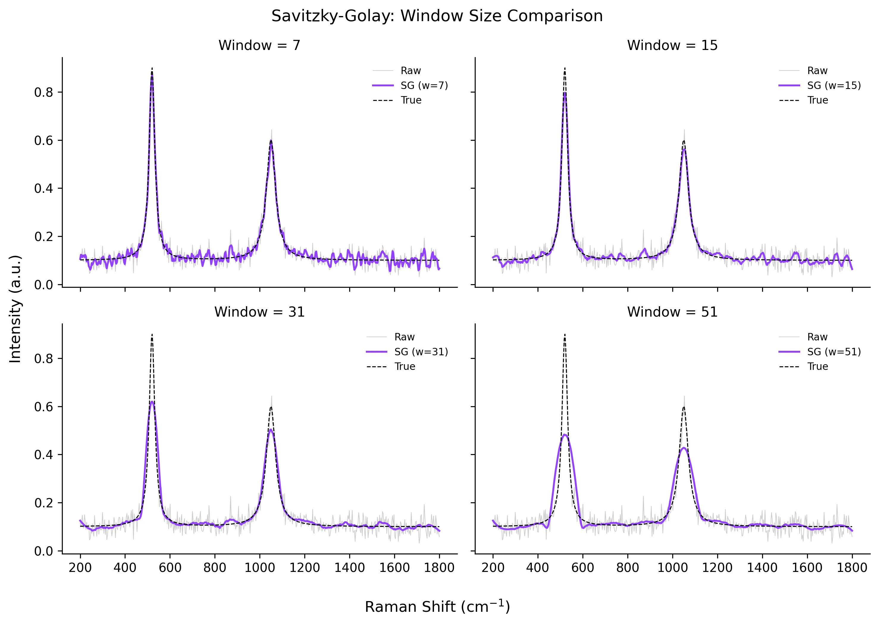
windows = [7, 15, 31, 51]
fig, axes = plt.subplots(2, 2, figsize=(10, 7), sharex=True, sharey=True)

for ax, w in zip(axes.flat, windows):
    y_sm = savgol_filter(y_noisy, window_length=w, polyorder=3)
    ax.plot(x, y_noisy, color='#cccccc', lw=0.5, label='Raw')
    ax.plot(x, y_sm, color='#9240ff', lw=1.5, label=f'SG (w={w})')
    ax.plot(x, y_clean, color='black', lw=0.8, ls='--', label='True')
    ax.set_title(f'Window = {w}', fontsize=11)
    ax.legend(frameon=False, fontsize=8)
    ax.spines[['top', 'right']].set_visible(False)

fig.supxlabel('Raman Shift (cm$^{-1}$)')
fig.supylabel('Intensity (a.u.)')
fig.suptitle('Savitzky-Golay: Window Size Comparison', fontsize=13)
plt.tight_layout()
plt.savefig('savgol_comparison.png', dpi=300, bbox_inches='tight')
plt.show()

Visualize This Code in Analyze

Derivative Calculation with Savitzky-Golay

One of the most powerful features of Savitzky-Golay filtering is its ability to compute smooth derivatives simultaneously with the smoothing step. The first derivative highlights inflection points and helps resolve overlapping peaks. The second derivative is widely used in near-infrared spectroscopy to remove baseline offsets and enhance spectral features.

import numpy as np
import matplotlib.pyplot as plt
from scipy.signal import savgol_filter

np.random.seed(42)
x = np.linspace(200, 1800, 500)
peak = 0.8 / (1 + ((x - 520) / 15) ** 2) + 0.5 / (1 + ((x - 1050) / 25) ** 2)
y_noisy = peak + 0.1 + np.random.normal(0, 0.02, size=x.shape)

y_smooth = savgol_filter(y_noisy, 21, 3, deriv=0)
y_d1     = savgol_filter(y_noisy, 21, 3, deriv=1, delta=(x[1]-x[0]))
y_d2     = savgol_filter(y_noisy, 21, 3, deriv=2, delta=(x[1]-x[0]))

fig, axes = plt.subplots(3, 1, figsize=(8, 7), sharex=True)
axes[0].plot(x, y_noisy, color='#ccc', lw=0.6)
axes[0].plot(x, y_smooth, color='#9240ff', lw=1.5)
axes[0].set_ylabel('Intensity')
axes[0].set_title('Smoothed Spectrum', fontsize=11)

axes[1].plot(x, y_d1, color='#9240ff', lw=1.2)
axes[1].axhline(0, color='gray', lw=0.5, ls='--')
axes[1].set_ylabel('1st Derivative')
axes[1].set_title('First Derivative (peak positions at zero crossings)', fontsize=11)

axes[2].plot(x, y_d2, color='#9240ff', lw=1.2)
axes[2].axhline(0, color='gray', lw=0.5, ls='--')
axes[2].set_ylabel('2nd Derivative')
axes[2].set_title('Second Derivative (peaks become minima)', fontsize=11)
axes[2].set_xlabel('Raman Shift (cm$^{-1}$)')

plt.tight_layout()
plt.savefig('savgol_derivatives.png', dpi=300, bbox_inches='tight')
plt.show()

Visualize This Advanced Variant

Common Errors and How to Fix Them

ValueError: window_length must be odd

Why: scipy.signal.savgol_filter requires an odd window_length because the local polynomial is centered on the middle point of the window.

Fix: Always use odd values: 5, 7, 9, 11, etc. If you compute the window programmatically, use w = w if w % 2 == 1 else w + 1.

Window length is larger than the data array

Why: If your signal has fewer points than the window_length, the filter cannot construct any local fit.

Fix: Ensure window_length < len(data). For very short signals, reduce the window size or use a different smoothing method.

polyorder must be less than window_length

Why: A polynomial of degree d requires at least d+1 points. If polyorder >= window_length, the system is underdetermined.

Fix: Use polyorder = 2 or 3 for most applications. Only increase it if you have very wide windows and sharp features.

Edge artifacts (smoothed curve deviates near boundaries)

Why: At the edges, the filter has fewer neighbouring points and must extrapolate the polynomial, leading to artefacts.

Fix: Trim the first and last (window_length // 2) points from the smoothed result, or use mode="nearest" or mode="wrap" if appropriate for your data.

Peaks are broadened or reduced after smoothing

Why: A window that is too wide or a polynomial order that is too low effectively acts as a moving average, distorting narrow peaks.

Fix: Reduce the window_length until peak height and width match the original. Compare the smoothed curve to a reference or repeat measurements.

Frequently Asked Questions

Apply Savitzky-Golay Smoothing in Python for Spectroscopy Data to Your Data

Upload your dataset and Plotivy generates the Python code, runs the analysis, and produces a publication-ready figure.

Generate Code for This Technique

Python Libraries