Peak Detection in Python with scipy.signal.find_peaks
Technique overview
Detect peaks in experimental data using scipy.signal.find_peaks. Covers prominence, height, threshold parameters with visualizations and peak area integration.
Peak detection is a building block for nearly every analytical pipeline that processes spectroscopic or chromatographic data. Whether you are identifying Raman bands in a mineral spectrum, counting action potentials in an electrophysiology recording, or locating retention-time peaks in a GC-MS chromatogram, scipy.signal.find_peaks is the go-to function. The challenge is not calling find_peaks itself - it is tuning the prominence, height, distance, and width parameters so that you capture the true peaks without false positives from noise or false negatives from broad features. This page demonstrates the parameter-tuning workflow with visual feedback and extends the analysis to peak area integration.
Key points
- Detect peaks in experimental data using scipy.signal.find_peaks. Covers prominence, height, threshold parameters with visualizations and peak area integration.
- Peak detection is a building block for nearly every analytical pipeline that processes spectroscopic or chromatographic data.
- Whether you are identifying Raman bands in a mineral spectrum, counting action potentials in an electrophysiology recording, or locating retention-time peaks in a GC-MS chromatogram, scipy.signal.find_peaks is the go-to function.
- The challenge is not calling find_peaks itself - it is tuning the prominence, height, distance, and width parameters so that you capture the true peaks without false positives from noise or false negatives from broad features.
Example Visualization
Review the example first, then use the live editor below to run and customize the full workflow.
Mathematical Foundation
Peak detection is a building block for nearly every analytical pipeline that processes spectroscopic or chromatographic data.
Equation
A peak at index i satisfies: x[i] > x[i-1] AND x[i] > x[i+1], subject to height, prominence, distance, and width constraints.Parameter breakdown
When to use this technique
Use find_peaks when your signal has clearly defined local maxima. Always start with prominence-based detection (robust to baseline drift) before fine-tuning with height and distance. For noisy data, smooth first with Savitzky-Golay, then detect peaks.
Apply This Technique Now
Run this analysis workflow with AI in seconds. Use the prepared technique prompt or bring your own dataset.
View example prompt
"Detect all peaks in my spectroscopy data, annotate them with height and width markers, and calculate the integrated area under each peak"
How to apply this technique in 30 seconds
Generate
Run the example prompt and let AI generate this technique automatically.
Refine and Export
Adjust code or prompt, then export publication-ready figures.
Implementation Code
The core data processing logic. Copy this block and replace the sample data with your measurements.
import numpy as np
from scipy.signal import find_peaks, peak_prominences, peak_widths

# --- Simulated chromatogram with 4 peaks ---
np.random.seed(42)
x = np.linspace(0, 20, 1000)  # minutes
signal = (0.6 * np.exp(-((x - 4.2) / 0.3) ** 2)
        + 1.0 * np.exp(-((x - 8.5) / 0.5) ** 2)
        + 0.3 * np.exp(-((x - 11.0) / 0.2) ** 2)
        + 0.8 * np.exp(-((x - 15.3) / 0.6) ** 2))
signal += np.random.normal(0, 0.02, size=x.shape)

# --- Detect peaks ---
peaks, properties = find_peaks(signal, height=0.1, prominence=0.05,
                                distance=20, width=3)

prominences = peak_prominences(signal, peaks)[0]
widths_result = peak_widths(signal, peaks, rel_height=0.5)

print(f"Found {len(peaks)} peaks:")
for i, pk in enumerate(peaks):
    print(f"  Peak {i+1}: time={x[pk]:.2f} min, height={signal[pk]:.3f}, "
f"prominence={prominences[i]:.3f}, width={widths_result[0][i]:.1f} pts")Visualization Code
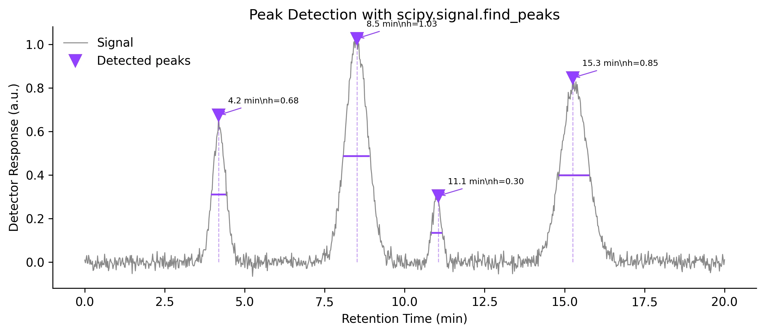
Complete matplotlib code for a publication-ready figure. Copy, paste into your notebook, and adjust labels to match your data.
import numpy as np
import matplotlib.pyplot as plt
from scipy.signal import find_peaks, peak_widths

np.random.seed(42)
x = np.linspace(0, 20, 1000)
signal = (0.6 * np.exp(-((x - 4.2) / 0.3) ** 2)
        + 1.0 * np.exp(-((x - 8.5) / 0.5) ** 2)
        + 0.3 * np.exp(-((x - 11.0) / 0.2) ** 2)
        + 0.8 * np.exp(-((x - 15.3) / 0.6) ** 2))
signal += np.random.normal(0, 0.02, size=x.shape)

peaks, props = find_peaks(signal, height=0.1, prominence=0.05,
                           distance=20, width=3)
widths_half = peak_widths(signal, peaks, rel_height=0.5)

fig, ax = plt.subplots(figsize=(9, 4))
ax.plot(x, signal, color='#888', lw=0.8, label='Signal')
ax.plot(x[peaks], signal[peaks], 'v', color='#9240ff', markersize=10,
        label='Detected peaks')

# Annotate each peak
for i, pk in enumerate(peaks):
    ax.vlines(x[pk], ymin=0, ymax=signal[pk], color='#9240ff',
              linestyle='--', lw=0.8, alpha=0.5)
    ax.annotate(f'{x[pk]:.1f} min\nh={signal[pk]:.2f}',
                xy=(x[pk], signal[pk]), xytext=(8, 10),
                textcoords='offset points', fontsize=7,
                arrowprops=dict(arrowstyle='->', color='#9240ff', lw=0.8))

# Width bars
ax.hlines(widths_half[1], x[widths_half[2].astype(int)],
          x[widths_half[3].astype(int)], color='#9240ff', lw=1.5)

ax.set_xlabel('Retention Time (min)')
ax.set_ylabel('Detector Response (a.u.)')
ax.set_title('Peak Detection with scipy.signal.find_peaks', fontsize=12)
ax.legend(frameon=False)
ax.spines[['top', 'right']].set_visible(False)
plt.tight_layout()
plt.savefig('peak_detection.png', dpi=300, bbox_inches='tight')
plt.show()Peak Area Integration (Trapezoidal Rule)
After detecting peaks, the next step in chromatography and spectroscopy is often to integrate the area under each peak. The trapezoidal rule (scipy.integrate.trapezoid) gives a quick, non-parametric area estimate. For overlapping peaks, deconvolution with Gaussian or Voigt models is preferred.
import numpy as np
import matplotlib.pyplot as plt
from scipy.signal import find_peaks, peak_widths
from scipy.integrate import trapezoid

np.random.seed(42)
x = np.linspace(0, 20, 1000)
signal = (0.6 * np.exp(-((x - 4.2) / 0.3) ** 2)
        + 1.0 * np.exp(-((x - 8.5) / 0.5) ** 2)
        + 0.3 * np.exp(-((x - 11.0) / 0.2) ** 2)
        + 0.8 * np.exp(-((x - 15.3) / 0.6) ** 2))
signal += np.random.normal(0, 0.02, size=x.shape)

peaks, _ = find_peaks(signal, height=0.1, prominence=0.05, distance=20)
widths_result = peak_widths(signal, peaks, rel_height=0.95)

fig, ax = plt.subplots(figsize=(9, 4))
ax.plot(x, signal, color='#888', lw=0.8)

colors = ['#9240ff', '#e67e22', '#27ae60', '#e74c3c']
for i, pk in enumerate(peaks):
    left = max(0, int(widths_result[2][i]))
    right = min(len(x) - 1, int(widths_result[3][i]))
    area = trapezoid(signal[left:right+1], x[left:right+1])
    ax.fill_between(x[left:right+1], signal[left:right+1],
                    alpha=0.3, color=colors[i % len(colors)])
    ax.annotate(f'Area = {area:.3f}', xy=(x[pk], signal[pk]),
                xytext=(0, 15), textcoords='offset points',
                ha='center', fontsize=8, color=colors[i % len(colors)])

ax.plot(x[peaks], signal[peaks], 'v', color='black', markersize=8)
ax.set_xlabel('Retention Time (min)')
ax.set_ylabel('Response')
ax.set_title('Peak Area Integration', fontsize=12)
ax.spines[['top', 'right']].set_visible(False)
plt.tight_layout()
plt.savefig('peak_areas.png', dpi=300, bbox_inches='tight')
plt.show()Common Errors and How to Fix Them
Too many false peaks detected (noise spikes)
Why: Using height as the only constraint picks up every noise spike above the threshold.
Fix: Add a prominence requirement (prominence=0.05 or higher) and a minimum distance between peaks. Smooth the data with Savitzky-Golay before detection.
Real peaks are missed (false negatives)
Why: The prominence or height threshold is set too high, or the distance constraint is too large, merging nearby peaks into one.
Fix: Lower the prominence threshold incrementally and visually inspect results. Reduce the distance parameter for closely spaced peaks.
Noisy baseline creates spurious peaks at the edges
Why: Baseline drift or edge artifacts from smoothing create apparent peaks near the start or end of the trace.
Fix: Crop the first and last few percent of the signal, or subtract the baseline before peak detection using scipy.signal.detrend or asymmetric least-squares.
Negative peaks (troughs) are not detected
Why: find_peaks only searches for local maxima. Absorption peaks (dips) are missed by default.
Fix: Invert the signal: peaks_neg, _ = find_peaks(-signal, ...). Alternatively, pass the negated signal and flip the results back.
Parameter tuning feels arbitrary and irreproducible
Why: There is no universally correct set of parameters - they depend on signal-to-noise ratio, peak shapes, and instrument resolution.
Fix: Document the exact parameter values used. Create a parameter sweep plot showing detected peaks vs parameter values. Use a validation dataset with known peaks.
Frequently Asked Questions
Learn More Before You Run It
Apply Peak Detection in Python with scipy.signal.find_peaks to Your Data
Upload your dataset and Plotivy generates the Python code, runs the analysis, and produces a publication-ready figure.
Generate Code for This TechniquePython Libraries
Quick Info
- Domain
- Signal Processing
- Typical Audience
- Spectroscopists, chromatographers, and electrophysiologists who need automated peak identification and quantification from instrument data