Mann-Whitney U Test in Python
Technique overview
Non-parametric alternative to the independent t-test for comparing two groups when data is not normally distributed, using rank-based methods.
The Mann-Whitney U test (also known as the Wilcoxon rank-sum test) is the standard non-parametric alternative to the independent-samples t-test. Because it operates on ranks rather than raw values, it makes no assumption about the underlying distribution of the data and is robust to outliers, skewed distributions, and ordinal measurements - conditions that are common in biological assays, clinical scores, and small-cohort studies. Whenever a Shapiro-Wilk normality test or Q-Q plot reveals that your two-group data deviates significantly from a Gaussian distribution, the Mann-Whitney U test is typically the most appropriate two-group comparison. This page covers the full workflow in Python using scipy.stats.mannwhitneyu, including effect size calculation and rank-based visualization.
Key points
- Non-parametric alternative to the independent t-test for comparing two groups when data is not normally distributed, using rank-based methods.
- The Mann-Whitney U test (also known as the Wilcoxon rank-sum test) is the standard non-parametric alternative to the independent-samples t-test.
- Because it operates on ranks rather than raw values, it makes no assumption about the underlying distribution of the data and is robust to outliers, skewed distributions, and ordinal measurements - conditions that are common in biological assays, clinical scores, and small-cohort studies.
- Whenever a Shapiro-Wilk normality test or Q-Q plot reveals that your two-group data deviates significantly from a Gaussian distribution, the Mann-Whitney U test is typically the most appropriate two-group comparison.
Example Visualization
Review the example first, then use the live editor below to run and customize the full workflow.
Mathematical Foundation
The Mann-Whitney U test (also known as the Wilcoxon rank-sum test) is the standard non-parametric alternative to the independent-samples t-test.
Equation
U = n1*n2 + n1*(n1+1)/2 - R1 (U statistic from rank sum R1)Parameter breakdown
When to use this technique
Use the Mann-Whitney U test when comparing two independent groups and the data is not normally distributed, is ordinal, or contains outliers that would unduly influence the mean. Do not use it as a general substitute for the t-test when normality is satisfied - the t-test is more powerful under normality. Also note that the Mann-Whitney U test correctly interprets as a test of stochastic dominance, not strictly a test of medians.
Apply This Technique Now
Run this analysis workflow with AI in seconds. Use the prepared technique prompt or bring your own dataset.
View example prompt
"Perform a Mann-Whitney U test on my two-group data, visualize the rank distributions as boxplots with significance annotation, and report the U statistic, p-value, and effect size (r = Z/sqrt(N))"
How to apply this technique in 30 seconds
Generate
Run the example prompt and let AI generate this technique automatically.
Refine and Export
Adjust code or prompt, then export publication-ready figures.
Implementation Code
The core data processing logic. Copy this block and replace the sample data with your measurements.
import numpy as np
from scipy import stats

# --- Simulated non-normal two-group data (e.g., clinical biomarker) ---
np.random.seed(42)
group_a = np.random.exponential(scale=3.0, size=25)   # right-skewed
group_b = np.random.exponential(scale=5.0, size=28)   # right-skewed, higher mean

# --- Normality check (Shapiro-Wilk) ---
_, p_norm_a = stats.shapiro(group_a)
_, p_norm_b = stats.shapiro(group_b)
print(f"Shapiro-Wilk p-value: Group A = {p_norm_a:.4f}, Group B = {p_norm_b:.4f}")
print("Note: p < 0.05 suggests non-normality -> Mann-Whitney appropriate\n")

# --- Mann-Whitney U test ---
u_stat, p_value = stats.mannwhitneyu(group_a, group_b, alternative='two-sided')
print(f"U statistic : {u_stat:.1f}")
print(f"p-value     : {p_value:.4f}")

# --- Effect size r = Z / sqrt(N) ---
n_total = len(group_a) + len(group_b)
# Convert U to Z-score using normal approximation
mean_u = len(group_a) * len(group_b) / 2
std_u = np.sqrt(len(group_a) * len(group_b) * (n_total + 1) / 12)
z_score = (u_stat - mean_u) / std_u
effect_size_r = z_score / np.sqrt(n_total)
print(f"Z-score     : {z_score:.4f}")
print(f"Effect size r = {effect_size_r:.4f} (|r|>0.5 = large)")

# --- Significance label ---
if p_value < 0.001:
    sig = '***'
elif p_value < 0.01:
    sig = '**'
elif p_value < 0.05:
    sig = '*'
else:
    sig = 'ns'
print(f"Significance: {sig}")Visualization Code
Complete matplotlib code for a publication-ready figure. Copy, paste into your notebook, and adjust labels to match your data.
import numpy as np
import matplotlib.pyplot as plt
from scipy import stats
# --- Data ---
np.random.seed(42)
group_a = np.random.exponential(scale=3.0, size=25)
group_b = np.random.exponential(scale=5.0, size=28)
u_stat, p_value = stats.mannwhitneyu(group_a, group_b, alternative='two-sided')
n_total = len(group_a) + len(group_b)
mean_u = len(group_a) * len(group_b) / 2
std_u = np.sqrt(len(group_a) * len(group_b) * (n_total + 1) / 12)
z_score = (u_stat - mean_u) / std_u
effect_r = z_score / np.sqrt(n_total)
sig = '***' if p_value < 0.001 else ('**' if p_value < 0.01 else ('*' if p_value < 0.05 else 'ns'))
fig, axes = plt.subplots(1, 2, figsize=(10, 5))
for ax in axes:
ax.spines['top'].set_visible(False)
ax.spines['right'].set_visible(False)
# Left: boxplot with individual data points
ax1 = axes[0]
bp = ax1.boxplot([group_a, group_b], patch_artist=True,
medianprops=dict(color='white', linewidth=2),
boxprops=dict(alpha=0.7),
widths=0.4)
colors = ['#9240ff', '#888888']
for patch, color in zip(bp['boxes'], colors):
patch.set_facecolor(color)
for i, (group, color) in enumerate(zip([group_a, group_b], colors), start=1):
jitter = np.random.uniform(-0.12, 0.12, size=len(group))
ax1.scatter(np.full(len(group), i) + jitter, group, s=18,
color=color, alpha=0.5, zorder=3)
# Significance bracket
y_max = max(group_a.max(), group_b.max())
bracket_h = y_max * 0.08
y_bracket = y_max + bracket_h
ax1.plot([1, 1, 2, 2], [y_bracket, y_bracket + bracket_h,
y_bracket + bracket_h, y_bracket],
color='white', linewidth=1.2)
ax1.text(1.5, y_bracket + bracket_h * 1.1, sig, ha='center', va='bottom',
fontsize=14, color='white', fontweight='bold')
ax1.set_xticks([1, 2])
ax1.set_xticklabels(['Group A', 'Group B'], fontsize=11)
ax1.set_ylabel('Biomarker Value', fontsize=11)
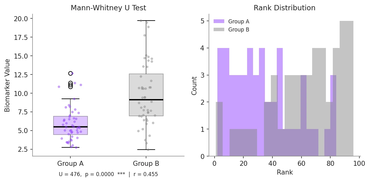
ax1.set_title('Mann-Whitney U Test', fontsize=12)
stats_text = (f'U = {u_stat:.0f}, p = {p_value:.4f}\n'
f'Effect size r = {effect_r:.3f}')
ax1.text(0.5, -0.18, stats_text, transform=ax1.transAxes,
ha='center', fontsize=9, color='#aaaaaa')
# Right: rank visualization
ax2 = axes[1]
all_vals = np.concatenate([group_a, group_b])
labels = ['A'] * len(group_a) + ['B'] * len(group_b)
ranks = stats.rankdata(all_vals)
rank_a = ranks[:len(group_a)]
rank_b = ranks[len(group_a):]
ax2.hist(rank_a, bins=15, alpha=0.6, color='#9240ff', label='Group A ranks',
density=True)
ax2.hist(rank_b, bins=15, alpha=0.6, color='#888888', label='Group B ranks',
density=True)
ax2.axvline(rank_a.mean(), color='#9240ff', linewidth=2, linestyle='--',
label=f'Mean rank A = {rank_a.mean():.1f}')
ax2.axvline(rank_b.mean(), color='#888888', linewidth=2, linestyle='--',
label=f'Mean rank B = {rank_b.mean():.1f}')
ax2.legend(frameon=False, fontsize=8)
ax2.set_xlabel('Rank', fontsize=11)
ax2.set_ylabel('Density', fontsize=11)
ax2.set_title('Rank Distributions', fontsize=12)
plt.tight_layout()
plt.savefig('mann_whitney_u_test.png', dpi=300, bbox_inches='tight')
plt.show()Paired Wilcoxon Signed-Rank Test for Matched Samples
When measurements are paired - for example before-vs-after treatment in the same subjects, or matched case-control pairs - use the Wilcoxon signed-rank test instead of the Mann-Whitney U test. This is the non-parametric analogue of the paired t-test and is more powerful than Mann-Whitney for paired designs because it accounts for within-subject correlation.
import numpy as np
import matplotlib.pyplot as plt
from scipy import stats

# --- Paired pre/post-treatment data ---
np.random.seed(42)
n = 20
pre  = np.random.exponential(scale=4.0, size=n)
post = pre * np.random.uniform(0.5, 0.9, size=n) + np.random.normal(0, 0.3, size=n)
post = np.clip(post, 0, None)

# --- Wilcoxon signed-rank test ---
stat, p_value = stats.wilcoxon(pre, post, alternative='two-sided')
sig = '***' if p_value < 0.001 else ('**' if p_value < 0.01 else ('*' if p_value < 0.05 else 'ns'))
print(f"Wilcoxon statistic: {stat:.1f},  p-value: {p_value:.4f}  ({sig})")

# --- Effect size r for Wilcoxon ---
z_approx = stats.norm.ppf(p_value / 2)  # approximate Z from p
effect_r = abs(z_approx) / np.sqrt(n)
print(f"Effect size r = {effect_r:.3f}")

# --- Paired point plot ---
fig, ax = plt.subplots(figsize=(5, 5))
ax.spines['top'].set_visible(False)
ax.spines['right'].set_visible(False)
for i in range(n):
    color = '#9240ff' if post[i] < pre[i] else '#888888'
    ax.plot([0, 1], [pre[i], post[i]], color=color, alpha=0.4, linewidth=1)
ax.scatter(np.zeros(n), pre, color='#888888', s=40, zorder=3, label='Pre')
ax.scatter(np.ones(n),  post, color='#9240ff', s=40, zorder=3, label='Post')
ax.set_xticks([0, 1])
ax.set_xticklabels(['Pre', 'Post'], fontsize=12)
ax.set_ylabel('Measurement Value', fontsize=11)
ax.set_title(f'Wilcoxon Signed-Rank Test\n{sig} (p = {p_value:.4f})', fontsize=12)
ax.legend(frameon=False, fontsize=9)
plt.tight_layout()
plt.savefig('wilcoxon_signed_rank.png', dpi=300, bbox_inches='tight')
plt.show()Common Errors and How to Fix Them
TypeError when calling mannwhitneyu with old scipy versions
Why: The alternative parameter ('two-sided', 'less', 'greater') was added in scipy 1.1.0. Older code that omitted it used the one-sided default, which can give incorrect results.
Fix: Always pass alternative='two-sided' explicitly unless you have a directional hypothesis. Update scipy to >= 1.7 with: pip install --upgrade scipy
p-value is identical whether using t-test or Mann-Whitney
Why: For large samples (n1, n2 > 25), both tests use a normal approximation and will give similar p-values. The difference matters most for small samples or heavily skewed data.
Fix: For small samples (n < 20 per group), use exact=True in mannwhitneyu to compute an exact p-value based on the permutation distribution rather than the normal approximation.
Reporting that Mann-Whitney tests whether medians are equal
Why: This is a common misconception. Mann-Whitney tests stochastic dominance: P(X > Y) = 0.5 under H0. It is only equivalent to a median test when the two distributions have the same shape.
Fix: Report the result as: "The Mann-Whitney U test indicated that group B values were stochastically greater than group A (U = X, p = Y)." Report medians as descriptive statistics separately.
Frequently Asked Questions
Apply Mann-Whitney U Test in Python to Your Data
Upload your dataset and Plotivy generates the Python code, runs the analysis, and produces a publication-ready figure.
Generate Code for This TechniquePython Libraries
Quick Info
- Domain
- Statistics
- Typical Audience
- Biologists and clinical researchers comparing two groups whose data violates normality assumptions or contains outliers that distort parametric tests