Menu

CLINICAL RESEARCH

Clinical Research Visualizations

From Kaplan-Meier curves and forest plots to CONSORT diagrams, swimmer plots, and NNT charts - create publication-ready clinical trial figures with AI-generated Python code.

or browse all example datasets

Essential Clinical Visualizations

Clinical trial data demands specialized visualizations - time-to-event analyses, treatment effect summaries, patient flow diagrams, and individual response tracking. Each requires rigorous statistical methodology and regulatory-compliant formatting.

Kaplan-Meier Curves

Survival probability estimates with confidence intervals and at-risk tables

Forest Plots

Meta-analysis effect sizes with confidence intervals and heterogeneity statistics

CONSORT Diagrams

Patient enrollment, randomization, and follow-up flow diagrams

Swimmer Plots

Individual patient treatment duration and response timelines

Waterfall Plots

Tumor response (% change from baseline) sorted by magnitude

Subgroup Analysis

Treatment effects across patient subgroups with interaction tests

Why Clinical Researchers Use Plotivy

Statistical Rigor

Kaplan-Meier log-rank tests, hazard ratios, and proper censoring marks generated automatically.

Regulatory Standards

CONSORT-compliant diagrams and ICH E9 guideline-ready statistical figures.

Interactive Exploration

Hover over individual patients in swimmer plots, drill into subgroup data.

Journal Formatting

Export to SVG/PDF sized for NEJM, Lancet, or JAMA column widths.

Kaplan-Meier Survival Analysis

Two-arm survival analysis with treatment vs control groups. The Kaplan-Meier estimator computes survival probabilities with 95% confidence intervals, censoring marks, and a number-at-risk table.

Forest Plot for Meta-Analysis

Eight clinical studies summarized with odds ratios and 95% confidence intervals. Study-level estimates are weighted by inverse variance, and the fixed-effect summary is shown as a diamond at the bottom.

Chart gallery

Explore Clinical Chart Types

Interactive examples with ready-to-run code

Browse all chart types →
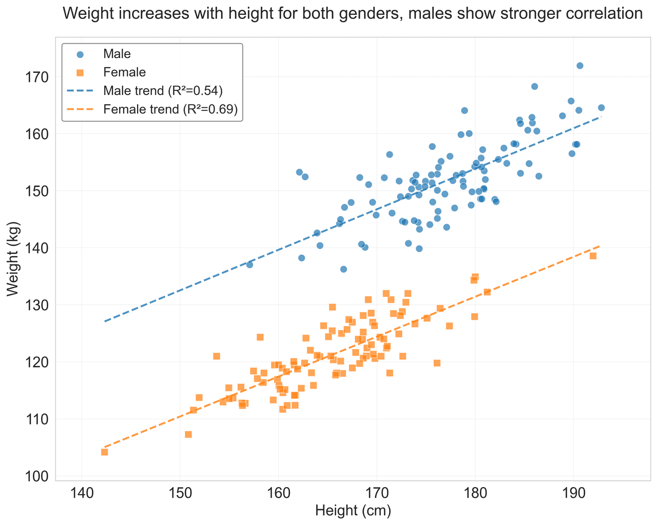
Scatter plot of height vs weight colored by gender with regression line
Statistical•matplotlib, seaborn
From the chart gallery•Correlation analysis between metrics

Scatterplot

Displays values for two variables as points on a Cartesian coordinate system.

Sample code / prompt

import matplotlib.pyplot as plt
import numpy as np
from scipy import stats
import pandas as pd

# Generate sample data
np.random.seed(42)
n_samples = 200
height = np.random.normal(170, 8, n_samples)
weight = height * 0.6 + np.random.normal(0, 8, n_samples) - 50
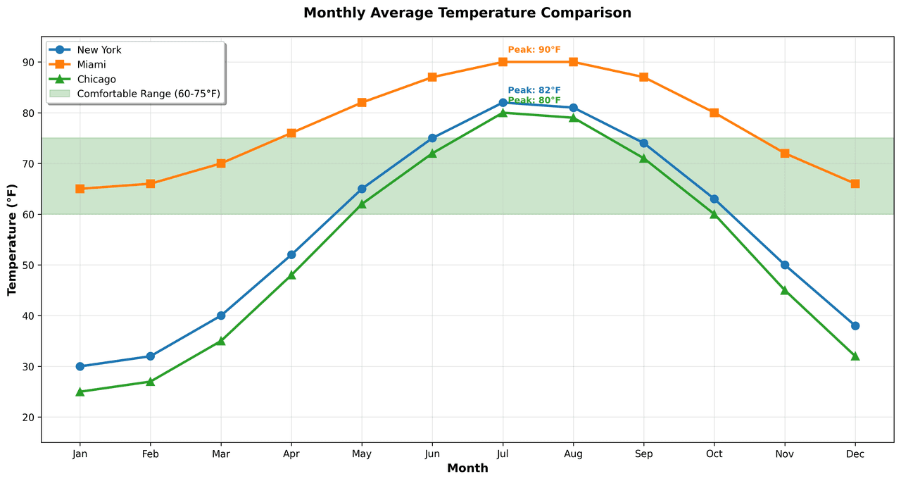
Multi-line graph showing temperature trends for 3 cities over a year
Time Series•matplotlib, seaborn
From the chart gallery•Stock price tracking over time

Line Graph

Displays data points connected by straight line segments to show trends over time.

Sample code / prompt

import matplotlib.pyplot as plt
import numpy as np

# Generate temperature data for 3 major US cities over 12 months
months = ['Jan', 'Feb', 'Mar', 'Apr', 'May', 'Jun', 'Jul', 'Aug', 'Sep', 'Oct', 'Nov', 'Dec']
nyc = [30, 32, 40, 52, 65, 75, 82, 81, 74, 63, 50, 38]
miami = [65, 66, 70, 76, 82, 87, 90, 90, 87, 80, 72, 66]
chicago = [25, 27, 35, 48, 62, 72, 80, 79, 71, 60, 45, 32]

# Create figure with enhanced styling
Box and whisker plot comparing gene expression across 4 genotypes with significance brackets
Distribution•seaborn, matplotlib
From the chart gallery•Comparing experimental groups in scientific research

Box and Whisker Plot

Displays data distribution using quartiles, median, and outliers in a standardized format.

Sample code / prompt

import numpy as np
import pandas as pd
import matplotlib.pyplot as plt
import seaborn as sns
from scipy import stats

# Generate gene expression data for 4 genotypes
np.random.seed(42)
genotypes = ['WT', 'KO1', 'KO2', 'Mutant']
n_per_group = 20
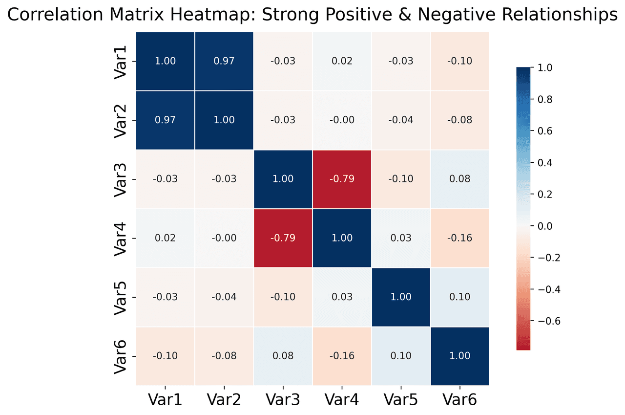
Correlation heatmap with diverging color scale and coefficient annotations
Statistical•seaborn, matplotlib
From the chart gallery•Correlation analysis between variables

Heatmap

Represents data values as colors in a two-dimensional matrix format.

Sample code / prompt

import matplotlib.pyplot as plt
import seaborn as sns
import pandas as pd
import numpy as np

# Create correlation matrix for financial metrics
metrics = ['Revenue', 'Profit', 'Expenses', 'ROI', 'Customers', 'AOV', 'Marketing', 'Employees']
correlation_data = np.array([
    [1.00, 0.85, -0.45, 0.72, 0.88, 0.65, 0.72, 0.55],
    [0.85, 1.00, -0.78, 0.92, 0.75, 0.58, 0.63, 0.48],
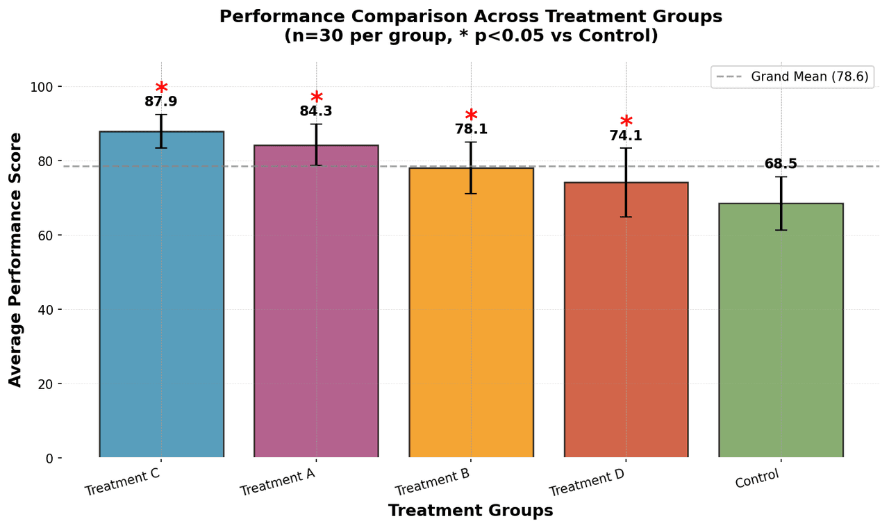
Bar chart comparing average scores across 5 groups with error bars
Comparison•matplotlib, seaborn
From the chart gallery•Comparing performance across categories

Bar Chart

Compares categorical data using rectangular bars with heights proportional to values.

Sample code / prompt

import numpy as np
import pandas as pd
import matplotlib.pyplot as plt
import seaborn as sns
from scipy import stats

# Generate performance scores for 5 treatment groups
np.random.seed(42)
groups = ['Control', 'Treatment A', 'Treatment B', 'Treatment C', 'Treatment D']
n_samples = 30

Ready to Visualize Your Clinical Data?

Upload your CSV, describe the plot you need, and get publication-ready clinical figures with full Python code in seconds.

Start Free - No Sign-Up