Biology Data Visualization: From Western Blots to Dose-Response Curves

Biology is messy. Unlike physics or chemistry where laws are often absolute, biological data is full of noise, variability, and outliers. If you have ever stared at a Western blot wondering how to turn it into a convincing bar chart, or spent hours fitting a dose-response curve that just would not cooperate - you are not alone.
This guide covers the essential plot types for biologists with live Python code editors you can modify and run instantly.
What You Will Learn
0.Live Code Lab: Dose-Response Curve
1.Dose-Response Curves (IC50/EC50)
2.Kaplan-Meier Survival Analysis
3.Western Blot Quantification
4.Gene Expression Heatmaps
5.Common Biology Mistakes
6.Live Code Lab: Survival Curves
0. Live Code Lab: Dose-Response Curve
This code fits a 4-parameter logistic (4PL) model to dose-response data and automatically calculates the IC50. It shows data points with SEM error bars and the fitted sigmoidal curve on a log-scale X-axis.
Modify the Hill coefficient, noise level, or IC50 value to see how the fit changes.
1. Dose-Response Curves (IC50/EC50)
Pharmacology and biochemistry rely heavily on dose-response curves. The key is fitting a 4-parameter logistic (4PL) or Hill equation to your data - but getting the fit right can be frustrating.
Log-Scale X-Axis
Always plot concentration logarithmically. Linear scale hides the sigmoidal shape and makes the IC50 impossible to read.
Show Replicates
Plot individual points (not just the mean) so reviewers can see the biological variability at each concentration.
Annotate IC50
Mark the IC50 directly on the plot with a dashed line and annotation arrow. Do not make readers eyeball it.
2. Kaplan-Meier Survival Analysis
For clinical trials or animal studies, Kaplan-Meier plots are the gold standard. They show the probability of survival (or any event) over time, and reviewers expect them to follow specific conventions.
Key Elements Reviewers Look For
- Censored data: Mark censored subjects with tick marks (|) on the curve - not circles or squares
- P-value: Include the log-rank test p-value directly on the plot
- Risk table: Align a "Number at Risk" table below the X-axis to show sample sizes
- Step function: Use
step()withwhere="post"- never smooth lines
Pro Tip
If you are comparing more than two groups, use Bonferroni correction for multiple comparisons and report the adjusted p-values. Many reviewers will reject papers that compare 3+ groups with pairwise log-rank tests without correction.
Try it
Try it now: turn this method into your next figure
Apply the same approach to your own dataset and generate clean, publication-ready code and plots in minutes.
Open in Plotivy Analyze →Newsletter
Get a weekly Python plotting tip
One concise tip each week for cleaner, faster scientific figures. Built for researchers who publish.
3. Western Blot Quantification
"Representative images" are great, but quantification is what convinces reviewers. The problem? Bar charts hide too much information when sample sizes are small (n < 10).
Do: Dot Plots with Error Bars
Overlay individual data points on top of mean +/- SEM. This shows exactly how many replicates you ran and the spread of the data - increasingly required by top journals.
Do Not: Plain Bar Charts
A bar chart with n=3 hides whether the effect is driven by one outlier. Nature, Cell, and PNAS all recommend showing individual data points when n < 10.
Try it: Upload your densitometry data and ask "Create a dot plot with error bars comparing protein expression between groups".
4. Gene Expression Heatmaps
When dealing with RNA-seq or microarray data, heatmaps are essential for visualizing clusters of up-regulated and down-regulated genes. But color choice can make or break your figure.
Colorblind-Safe Palettes
Avoid red-green color scales - about 8% of men are colorblind. Use a diverging Blue-White-Red or Purple-White-Orange scale instead.
Many journals now require colorblind-accessible figures. Using the right palette from the start saves revision headaches.
Clustering & Dendrograms
Hierarchical clustering with scipy.cluster.hierarchy reveals gene groups and sample relationships. Always show the dendrogram alongside your heatmap.
Z-score normalize your expression values before clustering so highly expressed genes do not dominate the visual.
5. Common Biology Visualization Mistakes
Bar charts for paired data
If you measured the same subject before and after treatment, use a paired line plot (slopegraph) instead of two bars. It shows the effect size much more clearly.
Hiding N
Always state the number of biological replicates (n) in the figure legend. Reviewers will ask for it if missing and they will note it during review.
Over-smoothing time series
Do not smooth line plots unless a mathematical model justifies it. Connect points with straight lines for time-series data.
Truncating Y-axes in bar charts
Starting the Y-axis above zero exaggerates small differences. If you need to show a small effect, use a dot plot with a broken axis instead.
Tired of formatting biology figures manually?
Describe your data in plain English and get publication-ready figures instantly. Plotivy handles dose-response fits, survival curves, and expression heatmaps automatically.
6. Live Code Lab: Kaplan-Meier Survival Curves
This code builds Kaplan-Meier curves from scratch - no lifelines or external stats library required. It handles censored observations (marked with tick marks) and compares two treatment groups.
Try changing the median survival times or the censoring rate to see how the curves shift.
Chart gallery
Biology-ready chart templates
Start from these gallery examples and customize for your dose-response, expression, or survival data.
.png&w=1280&q=70)
Box and Whisker Plot
Displays data distribution using quartiles, median, and outliers in a standardized format.
Sample code / prompt
import numpy as np
import pandas as pd
import matplotlib.pyplot as plt
import seaborn as sns
from scipy import stats

# Generate gene expression data for 4 genotypes
np.random.seed(42)
genotypes = ['WT', 'KO1', 'KO2', 'Mutant']
n_per_group = 20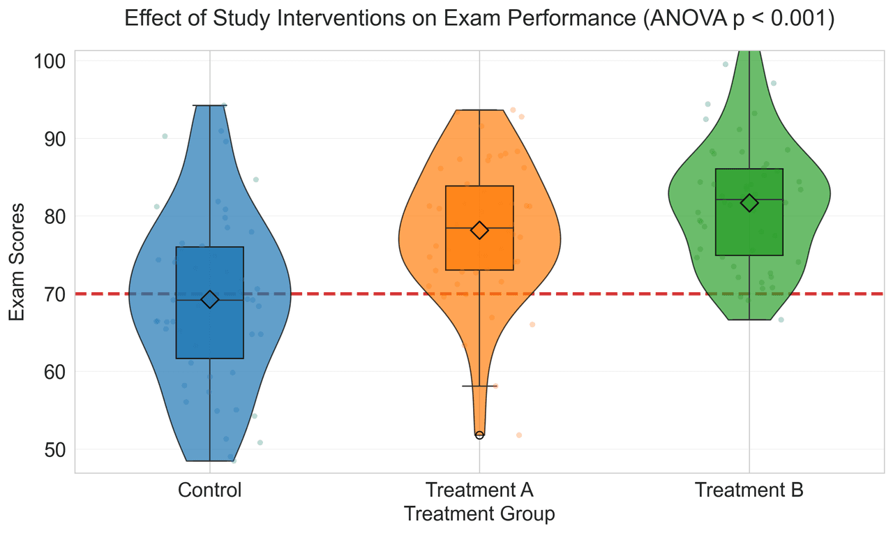
Violin Plot
Combines box plots with kernel density to show distribution shape across groups.
Sample code / prompt
import matplotlib.pyplot as plt
import seaborn as sns
import pandas as pd
import numpy as np
from scipy.stats import f_oneway

# Generate exam score data for 3 groups
np.random.seed(42)
control = np.random.normal(72, 12, 50)
treatment_a = np.random.normal(78, 10, 50)
Heatmap
Represents data values as colors in a two-dimensional matrix format.
Sample code / prompt
import matplotlib.pyplot as plt
import seaborn as sns
import pandas as pd
import numpy as np

# Create correlation matrix for financial metrics
metrics = ['Revenue', 'Profit', 'Expenses', 'ROI', 'Customers', 'AOV', 'Marketing', 'Employees']
correlation_data = np.array([
    [1.00, 0.85, -0.45, 0.72, 0.88, 0.65, 0.72, 0.55],
    [0.85, 1.00, -0.78, 0.92, 0.75, 0.58, 0.63, 0.48],
Error Bars
Graphical representations of the variability of data indicating error or uncertainty in measurements.
Sample code / prompt
import numpy as np
import matplotlib.pyplot as plt
from scipy import stats

# Generate bacterial growth data with replicates
np.random.seed(42)
time_points = np.array([0, 4, 8, 12, 18, 24])
mean_values = np.array([10, 25, 80, 250, 600, 800])

# Generate 5 replicates per time point with noiseVisualize Your Biology Data Now
Upload dose-response, survival, or expression data. Describe the plot you want and get publication-ready Python code instantly.
Technique guides scientists read next
scipy.signal.find_peaks guide
Tune prominence and width parameters for robust peak extraction.
Savitzky-Golay smoothing
Reduce noise while preserving peak shape and position.
PCA visualization workflow
Move from high-dimensional measurements to interpretable components.
ANOVA with post-hoc brackets
Add statistically correct pairwise significance annotations.
Found this helpful? Share it with your network.
Experimental Physicist & Photonics Researcher
Hands-on experience in silicon photonics, semiconductor fabrication (DRIE/ICP-RIE), optical simulation, and data-driven analysis. Built Plotivy to help researchers focus on discoveries instead of data struggles.
More about the authorVisualize your own data
Apply the techniques from this article to your own datasets. Upload CSV, Excel, or paste data directly.