Menu

Statistical Distribution Analysis

Publication-Ready Box Plots with Significance Brackets

Box plots are the gold standard for comparing distributions across groups. Plotivy generates them with automatic statistical tests, significance brackets, individual data point overlays, and journal-compliant styling.

Anatomy of a Box Plot

A box plot (box-and-whisker plot) summarizes a distribution using five key statistics. Understanding each element is crucial for interpreting your data correctly.

Median

Middle value (Q2) - the line inside the box

Q1 (25th)

Bottom of box - 25% of data falls below

Q3 (75th)

Top of box - 75% of data falls below

Whiskers

Extend to 1.5x IQR or data extremes

Outliers

Points beyond whiskers - always show them

Live Code Lab: Box Plot with Significance

This code creates a publication-ready box plot with ANOVA, pairwise t-tests, significance brackets (*, **, ***), and individual data point overlay. Edit anything and see results instantly.

Live Code Editor
Code EditorPython
Loading editor...
Live Preview

Preparing preview

Running once automatically on first load

Learn by Experimenting

This is a safe playground for learning! Try changing:

  • • Colors: Modify color values to see different palettes
  • • Numbers: Adjust sizes, positions, or data ranges
  • • Labels: Update titles, axis names, or legends

Edit the code, run it, then open the full data visualization tool to continue with your own dataset.

Key customization tips

  • Add more groups: extend the data and labels arrays
  • Change test: swap ttest_ind for mannwhitneyu for non-parametric data
  • Hide jitter: comment out the scatter loop to show boxes only
  • Horizontal layout: add vert=False to the boxplot call

Box Plot vs Alternatives

Plot TypeBest ForShowsLimitation
Box plotComparing 2-8 groupsMedian, IQR, outliersHides distribution shape
Violin plotDistribution shape mattersFull density + quartilesNeeds more space
Strip/jitter plotSmall sample sizes (n<30)Every individual pointCluttered for large n
Bar + error barsSimple group meansMean +/- SEM/SDHides distribution; avoid if possible

Pro tip: many journals now require showing individual data points on box plots. The code above already includes this via the jitter overlay.

Bonus: Grouped Box Plot for Time Series

Track biomarker changes across timepoints in a clinical trial or longitudinal study. Side-by-side panels show opposing trends clearly.

Live Code Editor
Code EditorPython
Loading editor...
Live Preview

Preparing preview

Running once automatically on first load

Learn by Experimenting

This is a safe playground for learning! Try changing:

  • • Colors: Modify color values to see different palettes
  • • Numbers: Adjust sizes, positions, or data ranges
  • • Labels: Update titles, axis names, or legends

Edit the code, run it, then open the full data visualization tool to continue with your own dataset.

Why Scientists Love Plotivy Box Plots

Auto significance testing

Plotivy runs ANOVA, t-tests, or Mann-Whitney automatically and adds the correct significance brackets to your plot.

Individual data overlay

Every data point is shown as a jittered dot overlaid on the box - meeting modern journal requirements.

Smart grouping

Upload grouped data and Plotivy detects categories, creating color-coded grouped box plots automatically.

Export-ready

300 DPI output with proper fonts, axis labels, and figure sizing ready for Nature, Science, or PLOS ONE.

Chart gallery

Related Statistical Charts

Explore more ways to visualize distributions

Browse all chart types →
Violin plot comparing score distributions across 3 groups with inner box plots
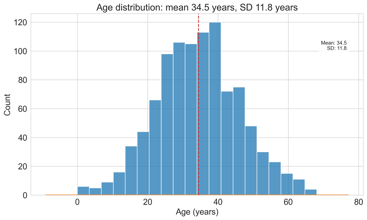
Distribution•seaborn, matplotlib
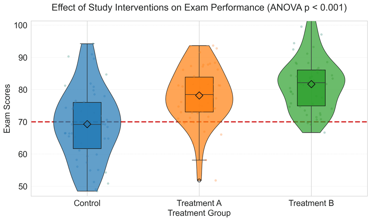
From the chart gallery•Comparing treatment effects across groups

Violin Plot

Combines box plots with kernel density to show distribution shape across groups.

Sample code / prompt

import matplotlib.pyplot as plt
import seaborn as sns
import pandas as pd
import numpy as np
from scipy.stats import f_oneway

# Generate exam score data for 3 groups
np.random.seed(42)
control = np.random.normal(72, 12, 50)
treatment_a = np.random.normal(78, 10, 50)
Bar chart comparing average scores across 5 groups with error bars
Comparison•matplotlib, seaborn
From the chart gallery•Comparing performance across categories

Bar Chart

Compares categorical data using rectangular bars with heights proportional to values.

Sample code / prompt

import numpy as np
import pandas as pd
import matplotlib.pyplot as plt
import seaborn as sns
from scipy import stats

# Generate performance scores for 5 treatment groups
np.random.seed(42)
groups = ['Control', 'Treatment A', 'Treatment B', 'Treatment C', 'Treatment D']
n_samples = 30
Scatter plot of height vs weight colored by gender with regression line
Statistical•matplotlib, seaborn
From the chart gallery•Correlation analysis between metrics

Scatterplot

Displays values for two variables as points on a Cartesian coordinate system.

Sample code / prompt

import matplotlib.pyplot as plt
import numpy as np
from scipy import stats
import pandas as pd

# Generate sample data
np.random.seed(42)
n_samples = 200
height = np.random.normal(170, 8, n_samples)
weight = height * 0.6 + np.random.normal(0, 8, n_samples) - 50
Histogram showing age distribution with 20 bins and KDE overlay
Distribution•matplotlib, seaborn
From the chart gallery•Analyzing age demographics

Histogram

Displays the distribution of numerical data by grouping values into bins.

Sample code / prompt

import matplotlib.pyplot as plt
import numpy as np
from scipy.stats import gaussian_kde, skewnorm

# Generate age data with slight right skew
np.random.seed(42)
ages = skewnorm.rvs(a=2, loc=42, scale=15, size=500)
ages = np.clip(ages, 18, 80)  # Clip to realistic range

fig, ax = plt.subplots(figsize=(12, 7))
Correlation heatmap with diverging color scale and coefficient annotations
Statistical•seaborn, matplotlib
From the chart gallery•Correlation analysis between variables

Heatmap

Represents data values as colors in a two-dimensional matrix format.

Sample code / prompt

import matplotlib.pyplot as plt
import seaborn as sns
import pandas as pd
import numpy as np

# Create correlation matrix for financial metrics
metrics = ['Revenue', 'Profit', 'Expenses', 'ROI', 'Customers', 'AOV', 'Marketing', 'Employees']
correlation_data = np.array([
    [1.00, 0.85, -0.45, 0.72, 0.88, 0.65, 0.72, 0.55],
    [0.85, 1.00, -0.78, 0.92, 0.75, 0.58, 0.63, 0.48],

Stop Making Box Plots the Hard Way

Upload your experimental data and get a publication-ready box plot with automatic statistics in under 30 seconds.