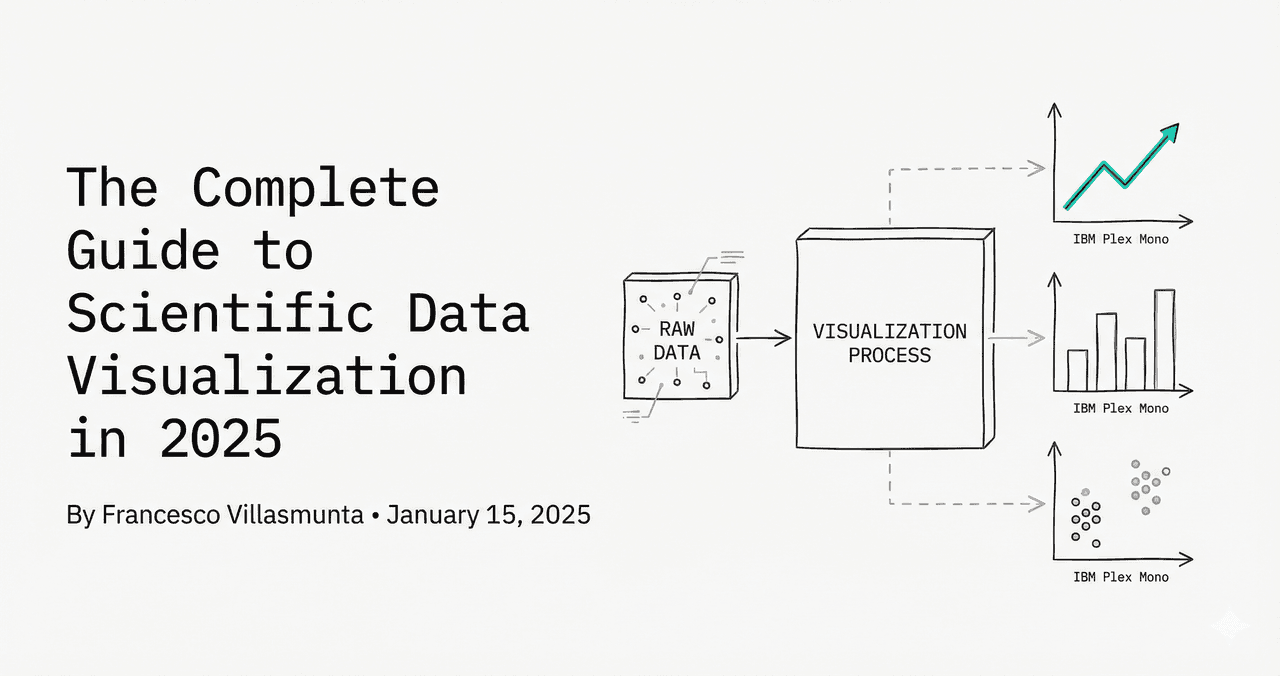
ggplot2 Color Palettes: How to Customize Colors in R Plots
Color is a primary aesthetic dimension in statistical graphs. In R's ggplot2, scale mapping controls color assignments. Correctly distinguishing color categories is essential to represent multiple experimental groups.
In This Guide
0.Live Code: Palette Customization
1.Discrete Manual Scales (scale_color_manual)
2.ColorBrewer Schemes (scale_fill_brewer)
3.Perceptually Uniform Gradients (scale_color_viridis_c)
4.Colorblind-Safe Design Best Practices
0. Live Code: Palette Customization
Palette transitions. Customize parameters using Python below, or upload your data to run R directly.
1. Discrete Manual Scales (scale_color_manual)
To specify exact hex codes for categorical factors, use scale_color_manual() for outlines and scale_fill_manual() for filled shapes:
R / ggplot2
# Manual discrete color mapping
ggplot(df, aes(x = group, y = measurement, color = treatment)) +
  geom_point() +
  scale_color_manual(values = c("Placebo" = "#94a3b8", "Drug A" = "#4f46e5", "Drug B" = "#059669"))
Try it
Try it now: turn this method into your next figure
Apply the same approach to your own dataset and generate clean, publication-ready code and plots in minutes.
Open in Plotivy Analyze →Newsletter
Get a weekly Python plotting tip
One concise tip each week for cleaner, faster scientific figures. Built for researchers who publish.
2. ColorBrewer Schemes (scale_fill_brewer)
Access pre-designed ColorBrewer palettes optimized for sequential, diverging, or qualitative variables:
R / ggplot2
# Qualitative ColorBrewer palette
ggplot(df, aes(x = group, y = measurement, fill = treatment)) +
  geom_col() +
  scale_fill_brewer(palette = "Set2")
3. Perceptually Uniform Gradients (scale_color_viridis_c)
For continuous variables, use viridis scales which map intensities uniformly:
R / ggplot2
# Continuous viridis scale
ggplot(df, aes(x = concentration, y = speed, color = temperature)) +
  geom_point() +
  scale_color_viridis_c(option = "plasma")
4. Colorblind-Safe Design Best Practices
Avoid pure red-green combinations. Utilize double encoding: represent groupings using different shapes and dashed lines alongside color changes.
Chart gallery
Explore related formats
Review visual formats.

Scatterplot
Displays values for two variables as points on a Cartesian coordinate system.
Sample code / prompt
import matplotlib.pyplot as plt
import numpy as np
from scipy import stats
import pandas as pd

# Generate sample data
np.random.seed(42)
n_samples = 200
height = np.random.normal(170, 8, n_samples)
weight = height * 0.6 + np.random.normal(0, 8, n_samples) - 50
Bar Chart
Compares categorical data using rectangular bars with heights proportional to values.
Sample code / prompt
import numpy as np
import pandas as pd
import matplotlib.pyplot as plt
import seaborn as sns
from scipy import stats

# Generate performance scores for 5 treatment groups
np.random.seed(42)
groups = ['Control', 'Treatment A', 'Treatment B', 'Treatment C', 'Treatment D']
n_samples = 30Build This Color-Mapped Plot Online
Upload your data and describe the design. Plotivy writes the ggplot2 code and executes it instantly.
Technique guides scientists read next
scipy.signal.find_peaks guide
Tune prominence and width parameters for robust peak extraction.
Savitzky-Golay smoothing
Reduce noise while preserving peak shape and position.
PCA visualization workflow
Move from high-dimensional measurements to interpretable components.
ANOVA with post-hoc brackets
Add statistically correct pairwise significance annotations.
Found this helpful? Share it with your network.
Experimental Physicist & Photonics Researcher
Hands-on experience in silicon photonics, semiconductor fabrication (DRIE/ICP-RIE), optical simulation, and data-driven analysis. Built Plotivy to help researchers focus on discoveries instead of data struggles.
More about the authorVisualize your own data
Apply the techniques from this article to your own datasets. Upload CSV, Excel, or paste data directly.