R ggplot2 Tutorial: Create Publication-Ready Figures in Minutes
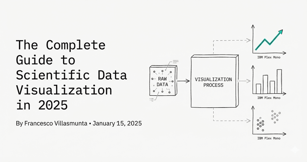
Creating publication-ready figures is a critical step in communicating scientific findings. R and the ggplot2 package provide one of the most powerful declarative systems for building statistical graphics. This guide walks you through the fundamentals of constructing a high-quality figure from scratch.
In This Tutorial
0.Live Code: Publication-Ready Plot
1.The ggplot2 Structure
2.Customizing Themes (theme_minimal)
3.Adding Custom Colors
4.Exporting to High-Resolution
0. Live Code: Publication-Ready Classic Style
Explore the clean, minimalist classic style equivalent to ggplot2's classic theme. Use the interactive editor below to customize parameters, or upload your data to run R directly.
1. The ggplot2 Grammar of Graphics Structure
The grammar of graphics separates data, aesthetics, and geometric layers. Here is the absolute baseline formula for any ggplot2 figure in R:
R / ggplot2
library(ggplot2)

# Baseline structure
ggplot(data = df, mapping = aes(x = variable_x, y = variable_y)) +
  geom_point() +
  geom_smooth(method = "lm")
2. Customizing Themes for Journals
Try it
Try it now: review your figure before submission
Upload your current plot and get an AI critique with concrete fixes for clarity, typography, color, and journal readiness.
Open AI Figure Reviewer →Newsletter
Get a weekly Python plotting tip
One concise tip each week for cleaner, faster scientific figures. Built for researchers who publish.
Default grey backgrounds are not suitable for journal submission. Utilize theme_classic() or theme_minimal() to establish a clean base:
R / ggplot2
ggplot(df, aes(x, y)) +
  geom_point() +
  theme_classic(base_size = 11, base_family = "Arial") +
  theme(
    panel.grid.major = element_blank(),
    panel.grid.minor = element_blank(),
    axis.line = element_line(size = 0.5, color = "black")
  )
3. Adding Custom Colors
Map qualitative variables using discrete scales with high-contrast, professional colors. Avoid generic primary colors:
R / ggplot2
ggplot(df, aes(x, y, color = group)) +
  geom_point(size = 2, alpha = 0.8) +
  scale_color_manual(values = c("#4f46e5", "#d97706", "#059669"))
4. Exporting to High-Resolution
Use ggsave() to export your plot. Standard journals require 300 DPI or higher:
R / ggplot2
p <- ggplot(df, aes(x, y)) + geom_point()
ggsave("figure1.png", plot = p, width = 120, height = 90, units = "mm", dpi = 300)
Chart gallery
Explore related formats
Review different plot formats where themes are crucial.

Scatterplot
Displays values for two variables as points on a Cartesian coordinate system.
Sample code / prompt
import matplotlib.pyplot as plt
import numpy as np
from scipy import stats
import pandas as pd

# Generate sample data
np.random.seed(42)
n_samples = 200
height = np.random.normal(170, 8, n_samples)
weight = height * 0.6 + np.random.normal(0, 8, n_samples) - 50
Line Graph
Displays data points connected by straight line segments to show trends over time.
Sample code / prompt
import matplotlib.pyplot as plt
import numpy as np

# Generate temperature data for 3 major US cities over 12 months
months = ['Jan', 'Feb', 'Mar', 'Apr', 'May', 'Jun', 'Jul', 'Aug', 'Sep', 'Oct', 'Nov', 'Dec']
nyc = [30, 32, 40, 52, 65, 75, 82, 81, 74, 63, 50, 38]
miami = [65, 66, 70, 76, 82, 87, 90, 90, 87, 80, 72, 66]
chicago = [25, 27, 35, 48, 62, 72, 80, 79, 71, 60, 45, 32]

# Create figure with enhanced styling
Bar Chart
Compares categorical data using rectangular bars with heights proportional to values.
Sample code / prompt
import numpy as np
import pandas as pd
import matplotlib.pyplot as plt
import seaborn as sns
from scipy import stats

# Generate performance scores for 5 treatment groups
np.random.seed(42)
groups = ['Control', 'Treatment A', 'Treatment B', 'Treatment C', 'Treatment D']
n_samples = 30.png&w=1280&q=70)
Box and Whisker Plot
Displays data distribution using quartiles, median, and outliers in a standardized format.
Sample code / prompt
import numpy as np
import pandas as pd
import matplotlib.pyplot as plt
import seaborn as sns
from scipy import stats

# Generate gene expression data for 4 genotypes
np.random.seed(42)
genotypes = ['WT', 'KO1', 'KO2', 'Mutant']
n_per_group = 20Build This Figure Online Instantly
Upload your dataset and toggle R language mode. Plotivy generates, runs, and renders ggplot2 code automatically.
Technique guides scientists read next
scipy.signal.find_peaks guide
Tune prominence and width parameters for robust peak extraction.
Savitzky-Golay smoothing
Reduce noise while preserving peak shape and position.
PCA visualization workflow
Move from high-dimensional measurements to interpretable components.
ANOVA with post-hoc brackets
Add statistically correct pairwise significance annotations.
Found this helpful? Share it with your network.
Experimental Physicist & Photonics Researcher
Hands-on experience in silicon photonics, semiconductor fabrication (DRIE/ICP-RIE), optical simulation, and data-driven analysis. Built Plotivy to help researchers focus on discoveries instead of data struggles.
More about the authorVisualize your own data
Apply the techniques from this article to your own datasets. Upload CSV, Excel, or paste data directly.