Recreating Famous Scientific Figures with AI

The best way to learn data visualization is to study the masters. This guide walks through recreating iconic scientific figures - from Anscombe's Quartet to modern multi-panel layouts - using Python and AI assistance.
In This Article
0.Live Code: Anscombe's Quartet
1.Why Recreate Famous Figures?
2.Gallery of Iconic Plots
3.Techniques for Modern Renditions
4.Try It Yourself
0. Live Code: Anscombe's Quartet
Four datasets, identical statistics, completely different patterns. Frank Anscombe published this in 1973 to demonstrate why you should always visualize your data before running statistics.
1. Why Recreate Famous Figures?
Learn Techniques
Each iconic figure teaches specific skills: multi-panel layouts, annotations, color theory, statistical overlays.
Build Portfolio
Recreations demonstrate technical skill. They show you understand both the data and the visualization principles.
Understand History
These figures changed science. Understanding why they were effective makes your own work better.
Try it
Try it now: turn this method into your next figure
Apply the same approach to your own dataset and generate clean, publication-ready code and plots in minutes.
Open in Plotivy Analyze →Newsletter
Get a weekly Python plotting tip
One concise tip each week for cleaner, faster scientific figures. Built for researchers who publish.
2. Gallery of Iconic Plots
Anscombe's Quartet (1973)
StatisticsBeginnerKey lesson: Always visualize data before computing summary statistics.
Minard's Napoleon March (1869)
InfographicsAdvancedKey lesson: Encode 6 dimensions (army size, location, direction, temperature, date, geography) in one figure.
John Snow's Cholera Map (1854)
EpidemiologyIntermediateKey lesson: Spatial visualization reveals patterns that tables cannot.
Gapminder Bubble Chart
Public HealthIntermediateKey lesson: Animation and size encoding reveal trends across time, income, and health.
Keeling Curve (1958-present)
Climate ScienceBeginnerKey lesson: Long time-series with seasonal decomposition tells a clear story.
Hertzsprung-Russell Diagram
AstrophysicsIntermediateKey lesson: Log-log scatter reveals stellar classification structure.
3. Techniques for Modern Renditions
Tips for faithful recreations
- Match the structure, not the pixels. Use the same chart type, axes, and data encoding. Modern styling is fine.
- Add a statistical overlay. The original may lack error bars, confidence intervals, or fit lines that modern standards require.
- Use subplots for comparison. Show the original concept (left) alongside your enhanced version (right).
- Document your code. Well-commented recreations are teaching tools. Explain why each design choice was made.
- Cite the original. Always reference the original paper and dataset in your figure caption.
Prompt template for recreations
Recreate [FIGURE NAME] from [AUTHOR, YEAR].
Use matplotlib with publication-quality styling.
- Match the original chart type and data encoding
- Add modern touches: clean spines, readable fonts
- Include a stats annotation box
- Export at 600 DPI for publication
4. Try It Yourself
Pick any famous figure from the gallery above, upload a relevant dataset, and describe what you want. Plotivy generates the Python code, you edit it until it matches, and export at publication resolution.
Chart gallery
Explore Chart Types
Every chart type you need to recreate iconic scientific figures.

Scatterplot
Displays values for two variables as points on a Cartesian coordinate system.
Sample code / prompt
import matplotlib.pyplot as plt
import numpy as np
from scipy import stats
import pandas as pd

# Generate sample data
np.random.seed(42)
n_samples = 200
height = np.random.normal(170, 8, n_samples)
weight = height * 0.6 + np.random.normal(0, 8, n_samples) - 50
Line Graph
Displays data points connected by straight line segments to show trends over time.
Sample code / prompt
import matplotlib.pyplot as plt
import numpy as np

# Generate temperature data for 3 major US cities over 12 months
months = ['Jan', 'Feb', 'Mar', 'Apr', 'May', 'Jun', 'Jul', 'Aug', 'Sep', 'Oct', 'Nov', 'Dec']
nyc = [30, 32, 40, 52, 65, 75, 82, 81, 74, 63, 50, 38]
miami = [65, 66, 70, 76, 82, 87, 90, 90, 87, 80, 72, 66]
chicago = [25, 27, 35, 48, 62, 72, 80, 79, 71, 60, 45, 32]

# Create figure with enhanced styling
Bar Chart
Compares categorical data using rectangular bars with heights proportional to values.
Sample code / prompt
import numpy as np
import pandas as pd
import matplotlib.pyplot as plt
import seaborn as sns
from scipy import stats

# Generate performance scores for 5 treatment groups
np.random.seed(42)
groups = ['Control', 'Treatment A', 'Treatment B', 'Treatment C', 'Treatment D']
n_samples = 30
Heatmap
Represents data values as colors in a two-dimensional matrix format.
Sample code / prompt
import matplotlib.pyplot as plt
import seaborn as sns
import pandas as pd
import numpy as np

# Create correlation matrix for financial metrics
metrics = ['Revenue', 'Profit', 'Expenses', 'ROI', 'Customers', 'AOV', 'Marketing', 'Employees']
correlation_data = np.array([
    [1.00, 0.85, -0.45, 0.72, 0.88, 0.65, 0.72, 0.55],
    [0.85, 1.00, -0.78, 0.92, 0.75, 0.58, 0.63, 0.48],
Contour Map
Displays three-dimensional data in two dimensions using contour lines connecting points of equal value.
Sample code / prompt
import matplotlib.pyplot as plt
import numpy as np

# Create electromagnetic field distribution in a rectangular waveguide
x = np.linspace(0, 10, 200)
y = np.linspace(0, 6, 120)
X, Y = np.meshgrid(x, y)

# TE10 mode in rectangular waveguide - dominant mode
# Electric field pattern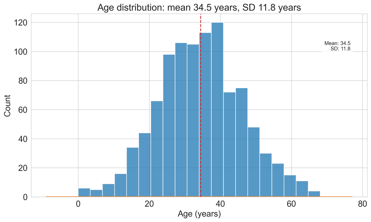
Histogram
Displays the distribution of numerical data by grouping values into bins.
Sample code / prompt
import matplotlib.pyplot as plt
import numpy as np
from scipy.stats import gaussian_kde, skewnorm

# Generate age data with slight right skew
np.random.seed(42)
ages = skewnorm.rvs(a=2, loc=42, scale=15, size=500)
ages = np.clip(ages, 18, 80)  # Clip to realistic range

fig, ax = plt.subplots(figsize=(12, 7))Recreate Any Figure with AI
Upload your data, describe the iconic figure you want to recreate, and edit the generated code.
Technique guides scientists read next
scipy.signal.find_peaks guide
Tune prominence and width parameters for robust peak extraction.
Savitzky-Golay smoothing
Reduce noise while preserving peak shape and position.
PCA visualization workflow
Move from high-dimensional measurements to interpretable components.
ANOVA with post-hoc brackets
Add statistically correct pairwise significance annotations.
Found this helpful? Share it with your network.
Experimental Physicist & Photonics Researcher
Hands-on experience in silicon photonics, semiconductor fabrication (DRIE/ICP-RIE), optical simulation, and data-driven analysis. Built Plotivy to help researchers focus on discoveries instead of data struggles.
More about the authorVisualize your own data
Apply the techniques from this article to your own datasets. Upload CSV, Excel, or paste data directly.