PhD Figure Hell: How to Make Publication-Ready Figures Without Losing Your Mind (or Your Weekend)

Every researcher has lived some version of this weekend. Figure formatting is not technically difficult - it is tedious, poorly documented, and unreasonably time-consuming. The gap between "I have a working plot in my Jupyter notebook" and "this is accepted by Nature" is about forty Stack Overflow tabs wide.

This guide is for you. We will walk through the five figure disasters that account for roughly 90% of formatting pain, give you the exact code to fix each one, and then talk honestly about how to build a workflow that does not steal your weekends.

The Five Figure Disasters (and How to Fix Them)

These are not edge cases. These are the reasons journals send back revision requests before anyone even reads your results section. Each one is easy to fix once you know where to look.

The Figure Workflow That Actually Works

The five fixes above solve individual problems. But the real time-saver is building a workflow that prevents those problems from appearing in the first place. After watching hundreds of researchers go through this process, here is what works:

Step 1: Sketch on Paper First

Before you open Python, grab a piece of paper and draw what you want the figure to communicate. Not how it should look - what story it tells. Which comparison matters? Where should the reader's eye go first? Ten minutes of sketching saves two hours of rearranging subplots.

Step 2: Pick the Right Tool for the Job

Matplotlib is powerful but verbose. Plotly is interactive but can be overkill for static journal figures. GraphPad Prism is familiar to biologists but limited in customization. The best tool is the one where you spend time thinking about your data instead of fighting the API. We are biased, obviously, but Plotivy was built specifically for this gap: researchers who know what they want but do not want to become Python developers to get it.

Step 3: Code It Once, Never Touch It Again

The single biggest mistake is making figures interactively - dragging elements around in a GUI, tweaking colors by eye, manually adjusting axis ranges. The moment your data changes (and it will change), you have to redo everything from scratch. Write a script. Save the script next to the data. When Reviewer 2 asks you to add a panel, you re-run the script with one modification instead of recreating the figure from memory. This is the core principle behind reproducible research figures.

Step 4: Export at Final Journal Specs from Day One

Do not wait until submission day to figure out the journal's requirements. Set your figsize, dpi, and font sizes at the start of the project according to your target journal. Single-column width is typically 3.3-3.5 inches, double-column is 6.5-7 inches. Bake these into a template script and reuse it across every figure in the paper.

Let Us Talk About Time

Here is arithmetic that nobody does until it is too late.

These numbers are not marketing fiction. They are based on what we hear from researchers every week. The formatting part - DPI, fonts, colors, legends, spacing - is where time vanishes. The scientific thinking part (choosing the right plot, deciding what to emphasize) takes the same amount of time regardless of the tool.

The Honest Recommendation

We built Plotivy, so take everything below with appropriate skepticism. But here is a genuinely honest assessment of when to use what.

Use GraphPad Prism if you are in biology or clinical research, your lab already has a license, and your figures are standard plot types (bar charts, survival curves, dose-response). Prism is excellent for what it does. Its limitations show up when you need unusual customization or when you want to automate figure generation across many datasets.

Use R with ggplot2 if you are in ecology, epidemiology, or any field where R is the standard. The grammar of graphics is beautiful once you learn it, and the ecosystem is unmatched for statistical visualization. The learning curve is real, though - budget a few weeks to become productive.

Use raw matplotlib/plotly if you genuinely enjoy programming, need extreme customization, or are building figures into an automated pipeline. You will have full control, and you will earn it through documentation-reading.

Use Plotivy if you know what figure you want but do not want to spend hours on formatting. If "make me a grouped bar chart with error bars, colorblind-safe colors, and Nature formatting" sounds like something you would rather say than code, that is exactly our use case. You describe the figure, Plotivy generates the Python code, and you get a publication-ready export in minutes. The generated code is yours - you can download it, modify it, and run it anywhere.

Chart gallery

PhD-Ready Chart Templates

Browse chart types with publication-quality defaults for your thesis.

Browse all chart types →

Comparison•matplotlib, seaborn

From the chart gallery•Comparing performance across categories

Bar Chart

Compares categorical data using rectangular bars with heights proportional to values.

Sample code / prompt

import numpy as np
import pandas as pd
import matplotlib.pyplot as plt
import seaborn as sns
from scipy import stats

# Generate performance scores for 5 treatment groups
np.random.seed(42)
groups = ['Control', 'Treatment A', 'Treatment B', 'Treatment C', 'Treatment D']
n_samples = 30

View chart detailsGenerate this chart

Distribution•matplotlib, seaborn

From the chart gallery•Analyzing age demographics

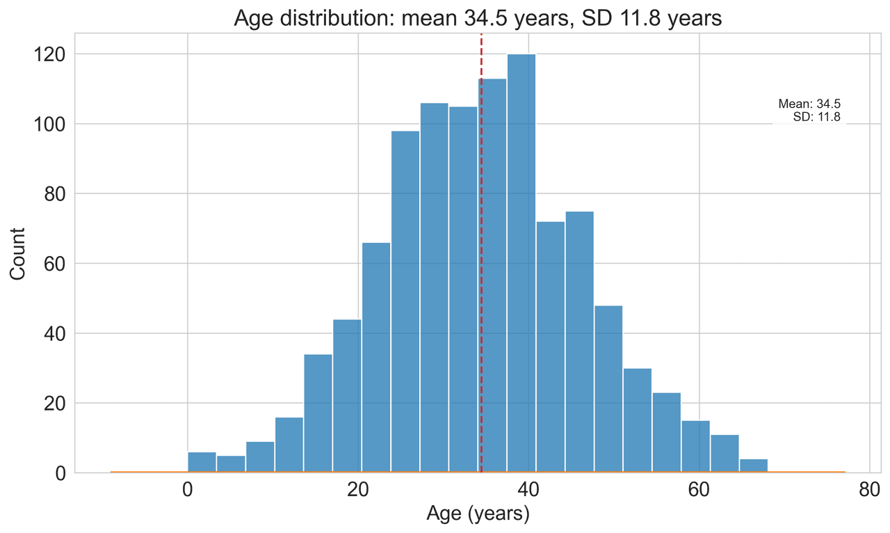
Histogram

Displays the distribution of numerical data by grouping values into bins.

Sample code / prompt

import matplotlib.pyplot as plt
import numpy as np
from scipy.stats import gaussian_kde, skewnorm

# Generate age data with slight right skew
np.random.seed(42)
ages = skewnorm.rvs(a=2, loc=42, scale=15, size=500)
ages = np.clip(ages, 18, 80)  # Clip to realistic range

fig, ax = plt.subplots(figsize=(12, 7))

View chart detailsGenerate this chart

Your Figures Should Not Be the Hard Part

You spent months - maybe years - collecting that data. The analysis was the hard part. The experimental design was the hard part. Exporting a plot at the correct DPI with readable fonts and a legend that does not cover your results should not be the thing that keeps you up at 3 AM.

Fix the five disasters above and you will eliminate most of the formatting pain immediately. Build a proper workflow and you will never have another figure emergency before a deadline. And if you want to skip the entire process and go straight from data to publication-ready figure, you know where to find us.

Good luck with the submission. You have got this.