Best Software for Scientific Plotting in 2026 (Ranked)

Choosing the right plotting software can save you hundreds of hours over the course of a PhD or research project. In 2026, the landscape has shifted from expensive desktop software to AI-powered web tools.
Here is our ranking of the best scientific plotting software available today, with a live code demo of the top-ranked tool.
Rankings Overview
0.Live Code Lab: Plotivy Demo
1.#1 Plotivy (AI-Powered)
2.#2 GraphPad Prism (Biology)
3.#3 OriginPro (Physics/Eng)
4.#4 R / ggplot2 (Power Users)
5.#5 Python / Matplotlib
6.Summary Comparison Table
0. Live Code Lab: What AI-Powered Plotting Looks Like
This is what Plotivy generates from a simple prompt: "Create a Michaelis-Menten fit of enzyme kinetics data with Vmax and Km annotations." Edit the code and run it yourself.
1. Plotivy
Editor's Choice - AI-Powered Scientific Plotting
#1Combines the flexibility of Python libraries with an intuitive AI interface. Real code, publication quality, free.
Why It Wins
- No coding required (but gives you the code)
- 100% free for academic usage
- Instant stats and detailed explanations
- Browser-based, no installation
- Journal-specific formatting presets
Considerations
- Newer ecosystem than legacy tools
- Requires internet connection
2. GraphPad Prism (Best for Biologists)
The Biologist's Favorite
Gold standard for basic biological statistics and plotting. Widely accepted in life sciences. For a direct migration path, see our GraphPad Prism alternative guide.
Strengths
- Excellent statistical guidance for bio assays
- Intuitive for standard dose-response experiments
- Widely accepted in life sciences journals
Limitations
- Expensive subscription ($$$)
- Rigid templates, limited customization
- Proprietary file format
3. OriginPro (Best for Physicists/Engineers)
Try it
Try it now: turn this method into your next figure
Apply the same approach to your own dataset and generate clean, publication-ready code and plots in minutes.
Open in Plotivy Analyze →Newsletter
Get a weekly Python plotting tip
One concise tip each week for cleaner, faster scientific figures. Built for researchers who publish.
The Powerhouse
Unparalleled depth for curve fitting and complex data analysis in physical sciences. We break down costs and alternatives in the OriginPro free alternative guide.
Strengths
- Extremely powerful analysis engine
- Handles massive datasets
- Highly customizable output
Limitations
- Very expensive ($$$$)
- Steep learning curve, cluttered interface
- Windows only
Why Pay Thousands for Software?
Plotivy gives you publication-quality figures with full code export - free for researchers.
Free account required - export publication-ready figures instantly.
4. R / ggplot2 (Best for Power Users)
Strengths
- Free and open-source
- Infinite customization
- Fully reproducible
- Rich statistical ecosystem
Limitations
- Requires coding proficiency
- Debugging can be time-consuming
- Slower for quick iterations
5. Python / Matplotlib / Seaborn
Strengths
- Free, integrates with AI/ML workflows
- Huge ecosystem (scipy, numpy, pandas)
- Modern standard for data science
- Supports advanced curve-fitting workflows and fast linear regression pipelines
Limitations
- Requires coding knowledge
- matplotlib syntax can be verbose
- Publication styling requires manual work
6. Summary Comparison Table
| Tool | Cost | Difficulty | Best For |
|---|---|---|---|
| Plotivy | Free | Low (AI) | Efficiency & Quality |
| GraphPad Prism | $$$ | Medium | Biology |
| OriginPro | $$$$ | High | Physics / Engineering |
| R / ggplot2 | Free | High (Code) | Statistics Power Users |
| Python / Matplotlib | Free | High (Code) | Data Science / ML |
Need concrete examples by chart family? Browse the full scientific chart index and jump directly into code templates.
Bottom Line
If you want the power of Python without the complexity, Plotivy is the answer. For biologists married to Prism or physicists who need OriginPro's curve fitting depth, those remain solid choices - but they come at a significant cost.
Chart gallery
50+ chart types supported
From basic scatter plots to complex 3D diagrams - all generated using standard Python libraries.

Scatterplot
Displays values for two variables as points on a Cartesian coordinate system.
Sample code / prompt
import matplotlib.pyplot as plt
import numpy as np
from scipy import stats
import pandas as pd

# Generate sample data
np.random.seed(42)
n_samples = 200
height = np.random.normal(170, 8, n_samples)
weight = height * 0.6 + np.random.normal(0, 8, n_samples) - 50
Bar Chart
Compares categorical data using rectangular bars with heights proportional to values.
Sample code / prompt
import numpy as np
import pandas as pd
import matplotlib.pyplot as plt
import seaborn as sns
from scipy import stats

# Generate performance scores for 5 treatment groups
np.random.seed(42)
groups = ['Control', 'Treatment A', 'Treatment B', 'Treatment C', 'Treatment D']
n_samples = 30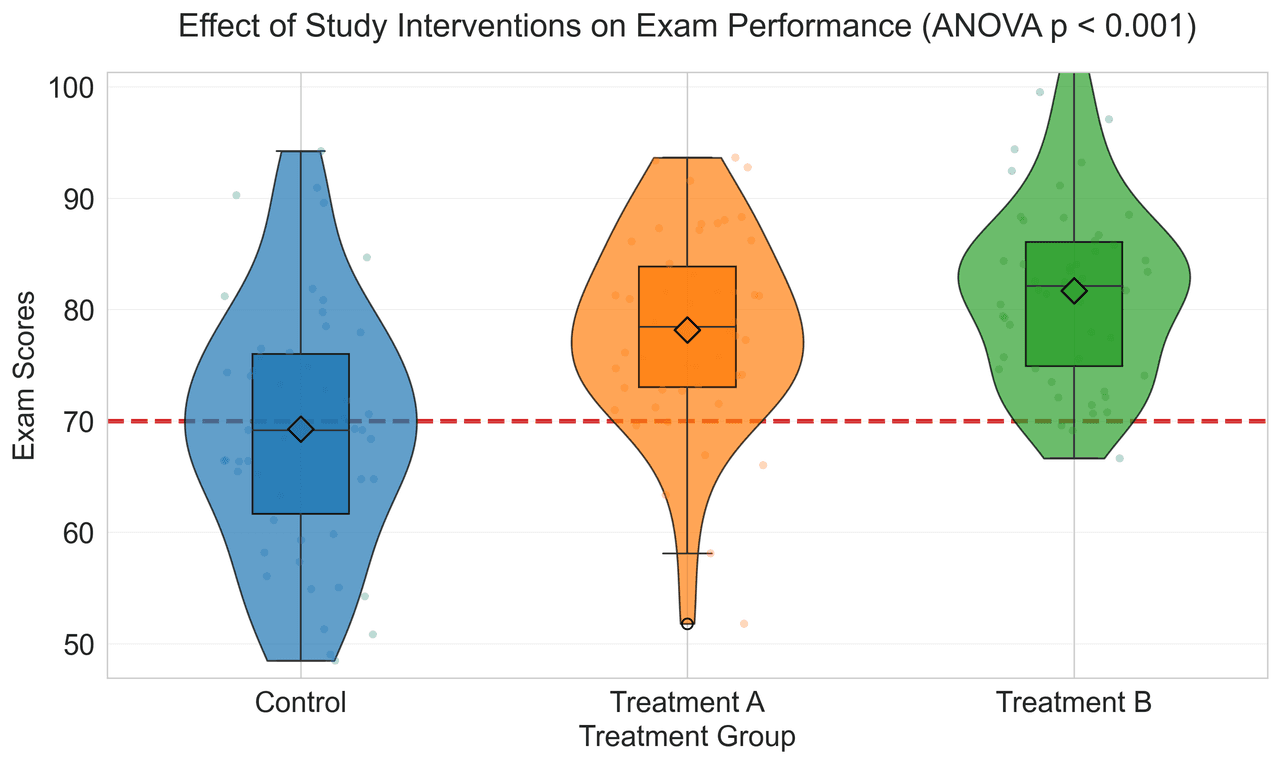
Violin Plot
Combines box plots with kernel density to show distribution shape across groups.
Sample code / prompt
import matplotlib.pyplot as plt
import seaborn as sns
import pandas as pd
import numpy as np
from scipy.stats import f_oneway

# Generate exam score data for 3 groups
np.random.seed(42)
control = np.random.normal(72, 12, 50)
treatment_a = np.random.normal(78, 10, 50)
Heatmap
Represents data values as colors in a two-dimensional matrix format.
Sample code / prompt
import matplotlib.pyplot as plt
import seaborn as sns
import pandas as pd
import numpy as np

# Create correlation matrix for financial metrics
metrics = ['Revenue', 'Profit', 'Expenses', 'ROI', 'Customers', 'AOV', 'Marketing', 'Employees']
correlation_data = np.array([
    [1.00, 0.85, -0.45, 0.72, 0.88, 0.65, 0.72, 0.55],
    [0.85, 1.00, -0.78, 0.92, 0.75, 0.58, 0.63, 0.48],
Radar Chart
Displays multivariate data on axes starting from a central point.
Sample code / prompt
import numpy as np
import matplotlib.pyplot as plt
from matplotlib.patches import Circle
import pandas as pd

# EV Model comparison data (0-100 scale)
categories = ['Range', 'Acceleration', 'Charging Speed',
              'Interior Quality', 'Technology', 'Value']
tesla_scores = [85, 90, 88, 70, 95, 80]
bmw_scores = [70, 80, 75, 90, 85, 65]
Sankey Diagram
Flow diagram where arrow widths are proportional to flow quantities.
Sample code / prompt
import plotly.graph_objects as go

# US Energy Flow Data (Quadrillion BTU)
sources = ['Coal', 'Natural Gas', 'Petroleum', 'Nuclear', 'Renewables']
source_values = [11, 32, 35, 8, 12]

transforms = ['Electricity Gen.', 'Direct Use', 'Rejected Energy']
end_uses = ['Residential', 'Commercial', 'Industrial', 'Transportation']

# Define flows: source -> transform/enduseFrequently Asked Questions
What is the best free software for scientific plotting?
Is OriginPro better than Python for scientific graphs?
Which plotting software do Nature and Science journals prefer?
Should I learn Python or R for scientific data visualization?
Can I create scientific plots without coding?
Stop Fighting with Complicated Software
Describe what you want and let Plotivy create the perfect figure in seconds. No installation, no subscription.
Free account required - start plotting instantly.
Technique guides scientists read next
scipy.signal.find_peaks guide
Tune prominence and width parameters for robust peak extraction.
Savitzky-Golay smoothing
Reduce noise while preserving peak shape and position.
PCA visualization workflow
Move from high-dimensional measurements to interpretable components.
ANOVA with post-hoc brackets
Add statistically correct pairwise significance annotations.
Found this helpful? Share it with your network.
Experimental Physicist & Photonics Researcher
Hands-on experience in silicon photonics, semiconductor fabrication (DRIE/ICP-RIE), optical simulation, and data-driven analysis. Built Plotivy to help researchers focus on discoveries instead of data struggles.
More about the authorVisualize your own data
Apply the techniques from this article to your own datasets. Upload CSV, Excel, or paste data directly.